Pearson and Lee's data on the heights of parents and children classified by gender

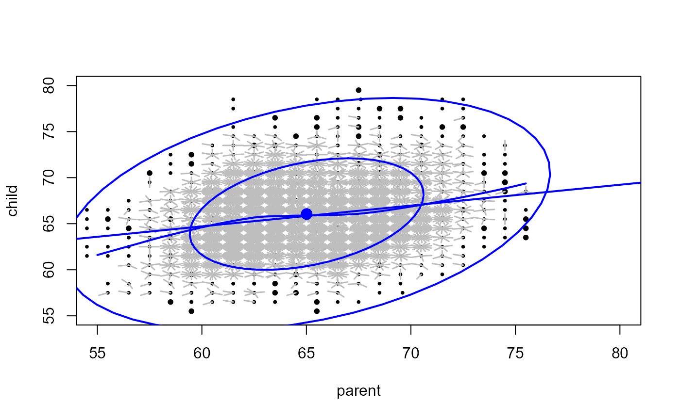
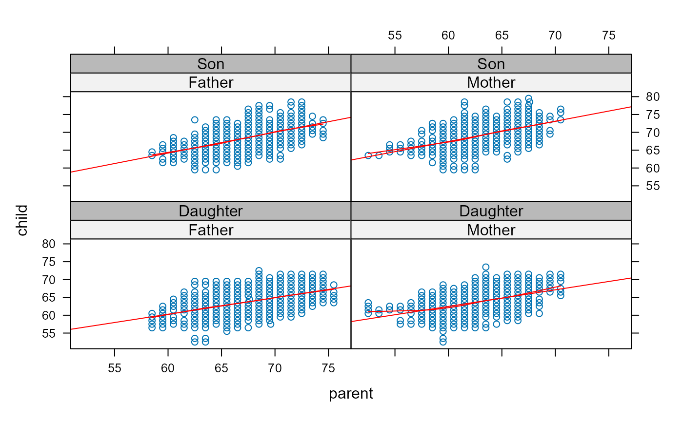
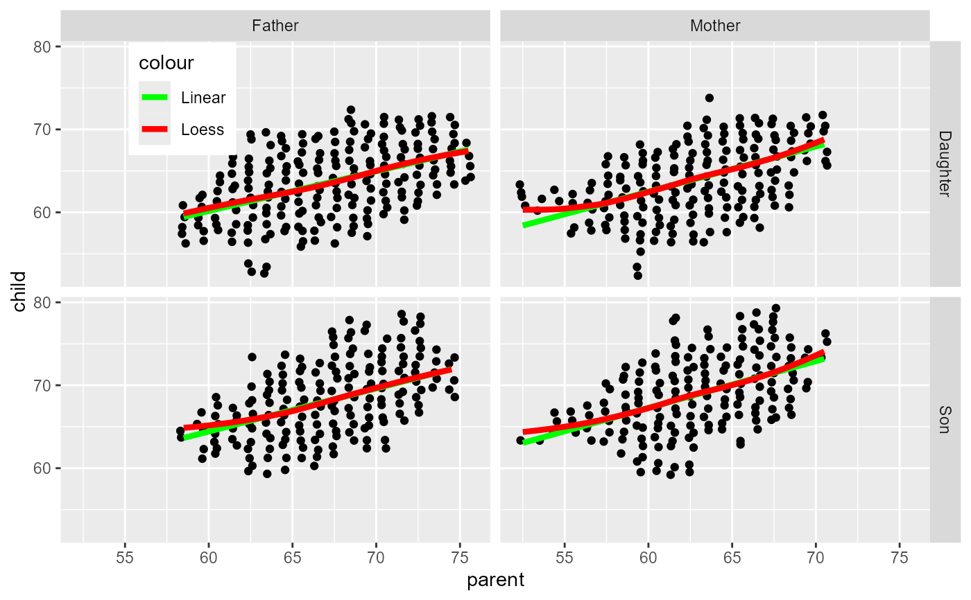
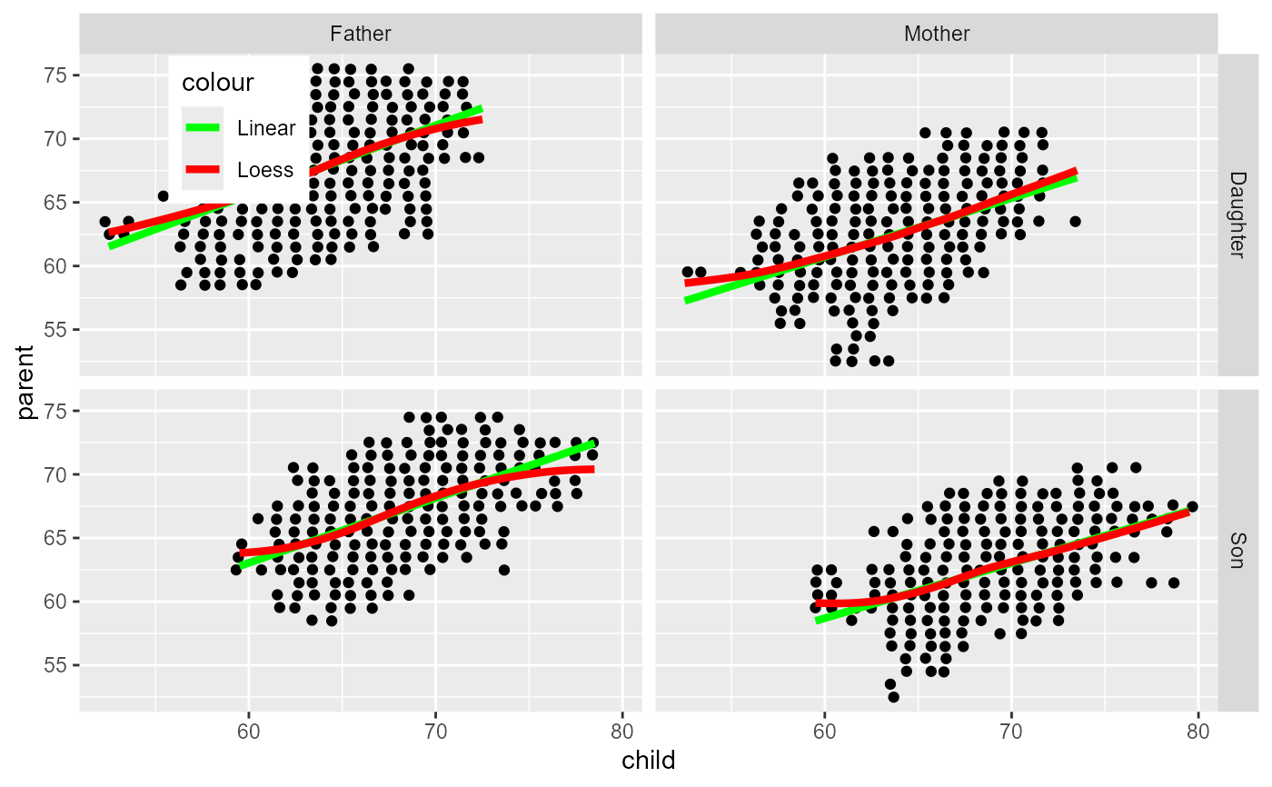
Wachsmuth et. al (2003) noticed that a loess smooth through Galton's data on heights of mid-parents and their offspring exhibited a slightly non-linear trend, and asked whether this might be due to Galton having pooled the heights of fathers and mothers and sons and daughters in constructing his tables and graphs.

To answer this question, they used analogous data from English families at about the same time, tabulated by Karl Pearson and Alice Lee (1896, 1903), but where the heights of parents and children were each classified by gender of the parent.

Usage

data(PearsonLee)

Format

A frequency data frame with 746 observations on the following 6 variables.

child: child height in inches, a numeric vector
parent: parent height in inches, a numeric vector
frequency: a numeric vector
gp: a factor with levels fd fs md ms
par: a factor with levels Father Mother
chl: a factor with levels Daughter Son

Details

The variables gp, par and chl are provided to allow stratifying the data according to the gender of the father/mother and son/daughter.

Source

Pearson, K. and Lee, A. (1896). Mathematical contributions to the theory of evolution. On telegony in man, etc. Proceedings of the Royal Society of London, 60 , 273-283.

Pearson, K. and Lee, A. (1903). On the laws of inheritance in man: I. Inheritance of physical characters. Biometika, 2(4), 357-462. (Tables XXII, p. 415; XXV, p. 417; XXVIII, p. 419 and XXXI, p. 421.)

References

Wachsmuth, A.W., Wilkinson L., Dallal G.E. (2003). Galton's bend: A previously undiscovered nonlinearity in Galton's family stature regression data. The American Statistician, 57, 190-192. https://www.cs.uic.edu/~wilkinson/Publications/galton.pdf

Examples

data(PearsonLee)
str(PearsonLee)
#> 'data.frame':	746 obs. of  6 variables:
#>  $ child    : num  59.5 59.5 59.5 60.5 60.5 61.5 61.5 61.5 61.5 61.5 ...
#>  $ parent   : num  62.5 63.5 64.5 62.5 66.5 59.5 60.5 62.5 63.5 64.5 ...
#>  $ frequency: num  0.5 0.5 1 0.5 1 0.25 0.25 0.5 1 0.25 ...
#>  $ gp       : Factor w/ 4 levels "fd","fs","md",..: 2 2 2 2 2 2 2 2 2 2 ...
#>  $ par      : Factor w/ 2 levels "Father","Mother": 1 1 1 1 1 1 1 1 1 1 ...
#>  $ chl      : Factor w/ 2 levels "Daughter","Son": 2 2 2 2 2 2 2 2 2 2 ...

with(PearsonLee, 
    {
    lim <- c(55,80)
    xv <- seq(55,80, .5)
    sunflowerplot(parent,child, number=frequency, xlim=lim, ylim=lim, seg.col="gray", size=.1)
    abline(lm(child ~ parent, weights=frequency), col="blue", lwd=2)
    lines(xv, predict(loess(child ~ parent, weights=frequency), data.frame(parent=xv)), 
          col="blue", lwd=2)
    # NB: dataEllipse doesn't take frequency into account
    if(require(car)) {
    dataEllipse(parent,child, xlim=lim, ylim=lim, plot.points=FALSE)
        }
  })


## separate plots for combinations of (chl, par)

# this doesn't quite work, because xyplot can't handle weights
require(lattice)
xyplot(child ~ parent|par+chl, data=PearsonLee, type=c("p", "r", "smooth"), col.line="red")


# Using ggplot [thx: Dennis Murphy]
require(ggplot2)
ggplot(PearsonLee, aes(x = parent, y = child, weight=frequency)) +
   geom_point(size = 1.5, position = position_jitter(width = 0.2)) +
   geom_smooth(method = lm, aes(weight = PearsonLee$frequency,
               colour = 'Linear'), se = FALSE, size = 1.5) +
   geom_smooth(aes(weight = PearsonLee$frequency,
               colour = 'Loess'), se = FALSE, size = 1.5) +
   facet_grid(chl ~ par) +
   scale_colour_manual(breaks = c('Linear', 'Loess'),
                       values = c('green', 'red')) +
   theme(legend.position = c(0.14, 0.885),
        legend.background = element_rect(fill = 'white'))
#> Warning: A numeric `legend.position` argument in `theme()` was deprecated in ggplot2
#> 3.5.0.
#> ℹ Please use the `legend.position.inside` argument of `theme()` instead.
#> Warning: Use of `PearsonLee$frequency` is discouraged.
#> ℹ Use `frequency` instead.
#> Warning: Use of `PearsonLee$frequency` is discouraged.
#> ℹ Use `frequency` instead.
#> `geom_smooth()` using formula = 'y ~ x'
#> `geom_smooth()` using method = 'loess' and formula = 'y ~ x'


# inverse regression, as in Wachmuth et al. (2003)

ggplot(PearsonLee, aes(x = child, y = parent, weight=frequency)) +
   geom_point(size = 1.5, position = position_jitter(width = 0.2)) +
   geom_smooth(method = lm, aes(weight = PearsonLee$frequency,
               colour = 'Linear'), se = FALSE, size = 1.5) +
   geom_smooth(aes(weight = PearsonLee$frequency,
               colour = 'Loess'), se = FALSE, size = 1.5) +
   facet_grid(chl ~ par) +
   scale_colour_manual(breaks = c('Linear', 'Loess'),
                       values = c('green', 'red')) +
   theme(legend.position = c(0.14, 0.885),
        legend.background = element_rect(fill = 'white'))
#> Warning: Use of `PearsonLee$frequency` is discouraged.
#> ℹ Use `frequency` instead.
#> Warning: Use of `PearsonLee$frequency` is discouraged.
#> ℹ Use `frequency` instead.
#> `geom_smooth()` using formula = 'y ~ x'
#> `geom_smooth()` using method = 'loess' and formula = 'y ~ x'