Code
library(ggplot2)
library(dplyr)
library(arrangements)
library(moments)From the time, long ago, I first studied linear algebra, I’ve always had a fascination with the idea of the determinant of a square matrix, \(\text{det}(\mathbf{A}) \equiv | \mathbf{A} |\). You just take your matrix \(\mathbf{A}\), which could be \((2 \times 2)\), or \((10 \times 10)\), or \((100 \times 100)\), … and \(| \mathbf{A} |\) turns that into a single number, that expresses many of it’s properties—algebraic, geometric and statistical.
In short, the determinant \(| \mathbf{A} |\) is a measure of the “size” of \(\mathbf{A}\).
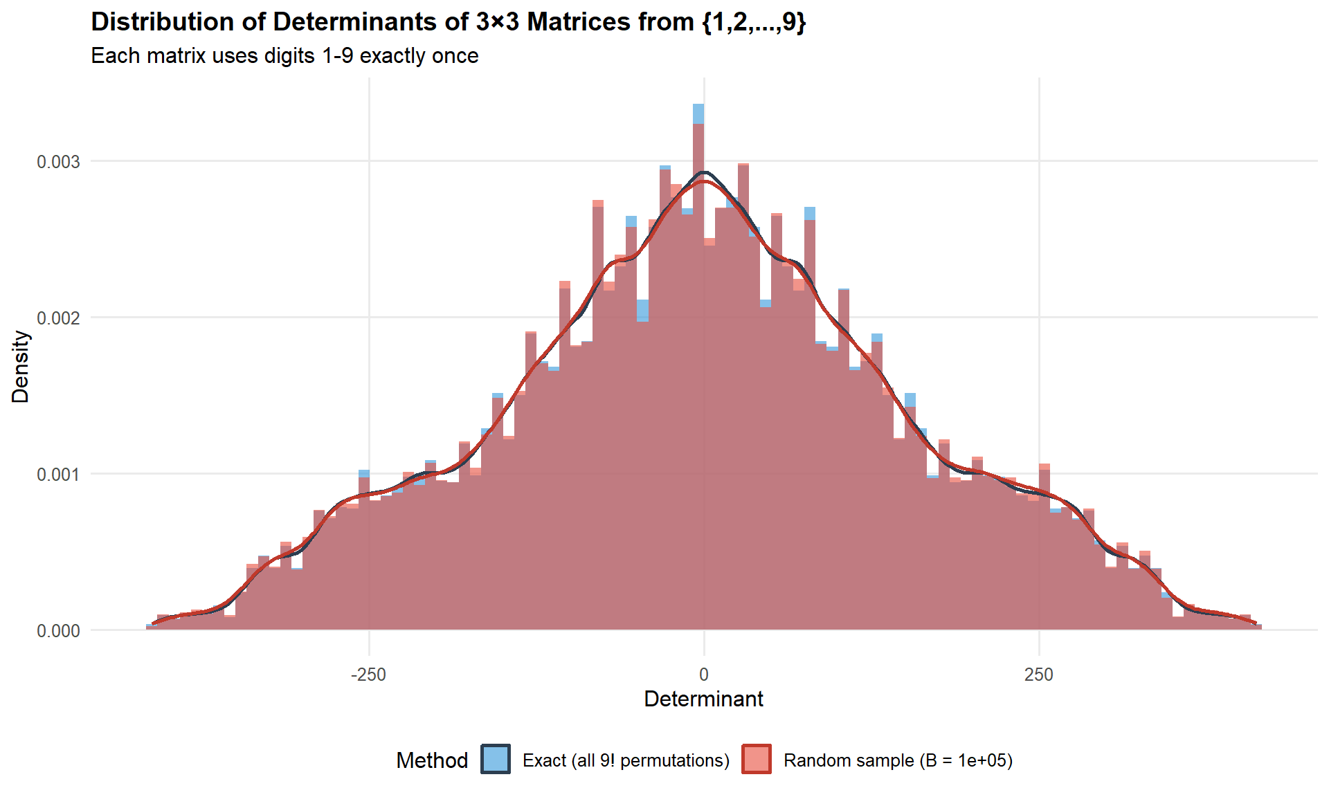
This post explores an interesting combinatorial and statistical problem: What is the distribution of determinants of all 3×3 matrices that can be formed from the numbers 1 through 9, each used exactly once? It arose from a simpler question Math StackExchange: What is the total number 3x3 matrices using only digits 1 to 9?
We answer this question in two ways:
library(ggplot2)
library(dplyr)
library(arrangements)
library(moments)\(9! = 362,880\) is a large number, but no so large to preclude an elegant two-line computational solution, even if it takes time and storage space.
arrangements::permutations() to generate all of theseapply() to calculate their determinants, with a helper function det_from_vec()Computing exact distribution using all 362,880 permutations of the digits 1-9.
det_from_vec <- function(v) {
  M <- matrix(v, nrow = 3, ncol = 3, byrow = TRUE)
  det(M)
}

all_perms <- arrangements::permutations(1:9, k = 9)
determinants_exact <- apply(all_perms, 1, det_from_vec)Generating a Monte Carlo approximation with a large random sample of permutations.
B <- 100000
set.seed(42)

determinants_random <- replicate(B, {
  v <- sample(1:9, 9, replace = FALSE)
  det_from_vec(v)
})if (!is.null(determinants_exact)) {
cat("EXACT SOLUTION (all 9! permutations):\n")
cat(sprintf(" Total permutations: %d\n", length(determinants_exact)))
cat(sprintf(" Range: [%.1f, %.1f]\n",
min(determinants_exact), max(determinants_exact)))
cat(sprintf(" Mean: %.2f\n", mean(determinants_exact)))
cat(sprintf(" Median: %.2f\n", median(determinants_exact)))
cat(sprintf(" SD: %.2f\n", sd(determinants_exact)))
cat(sprintf(" Unique values: %d\n", length(unique(determinants_exact))))
n_zero <- sum(determinants_exact == 0)
cat(sprintf(" Zero determinants: %d (%.2f%%)\n",
n_zero, 100 * n_zero / length(determinants_exact)))
}EXACT SOLUTION (all 9! permutations):
Total permutations: 362880
Range: [-412.0, 412.0]
Mean: -0.00
Median: 0.00
SD: 154.85
Unique values: 3891
Zero determinants: 1488 (0.41%)cat("RANDOM PERMUTATION SAMPLE (B =", B, "):\n")RANDOM PERMUTATION SAMPLE (B = 1e+05 ):cat(sprintf(" Range: [%.1f, %.1f]\n",
min(determinants_random), max(determinants_random))) Range: [-412.0, 412.0]cat(sprintf(" Mean: %.2f\n", mean(determinants_random))) Mean: 0.05cat(sprintf(" Median: %.2f\n", median(determinants_random))) Median: 0.00cat(sprintf(" SD: %.2f\n", sd(determinants_random))) SD: 155.43cat(sprintf(" Unique values: %d\n", length(unique(determinants_random)))) Unique values: 3451if (!is.null(determinants_exact)) {
df_combined <- rbind(
data.frame(determinant = determinants_exact,
method = "Exact (all 9! permutations)"),
data.frame(determinant = determinants_random,
method = paste0("Random sample (B = ", format(B, big.mark = ","), ")"))
)
ggplot(df_combined, aes(x = determinant, fill = method)) +
geom_histogram(aes(y = after_stat(density)),
bins = 100, alpha = 0.6, position = "identity") +
geom_density(aes(color = method), linewidth = 1, fill = NA) +
scale_fill_manual(values = c("#3498db", "#e74c3c")) +
scale_color_manual(values = c("#2c3e50", "#c0392b")) +
labs(
title = "Distribution of Determinants of 3×3 Matrices from {1,2,...,9}",
subtitle = "Each matrix uses digits 1-9 exactly once",
x = "Determinant", y = "Density", fill = "Method", color = "Method"
) +
theme_minimal(base_size = 12) +
theme(legend.position = "bottom",
plot.title = element_text(face = "bold", size = 14),
panel.grid.minor = element_blank())
}
if (!is.null(determinants_exact)) {
ggplot(data.frame(determinant = determinants_exact), aes(x = determinant)) +
geom_histogram(aes(y = after_stat(density)),
bins = 120, fill = "#3498db", alpha = 0.7) +
geom_density(color = "#2c3e50", linewidth = 1.2) +
labs(
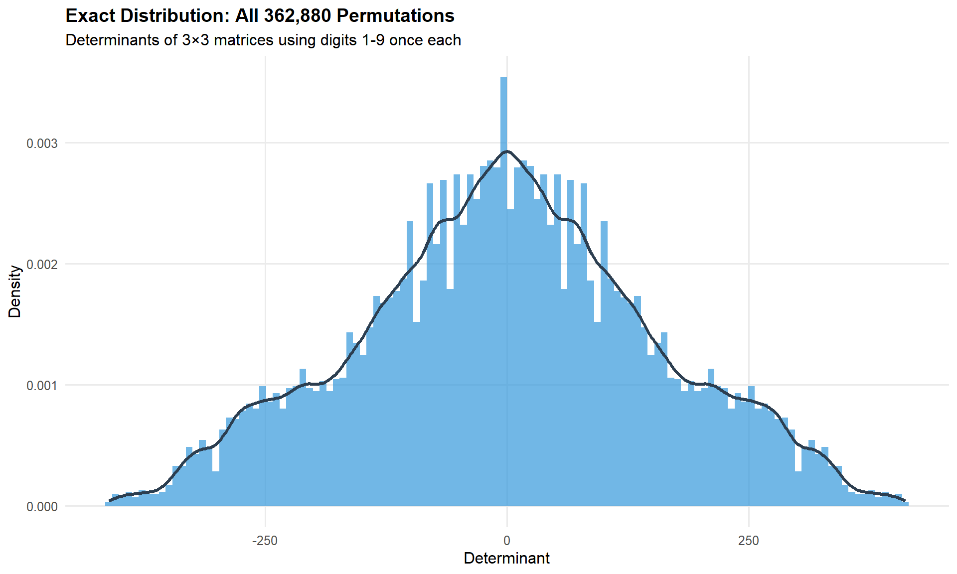
title = "Exact Distribution: All 362,880 Permutations",
subtitle = "Determinants of 3×3 matrices using digits 1-9 once each",
x = "Determinant", y = "Density"
) +
theme_minimal(base_size = 12) +
theme(plot.title = element_text(face = "bold", size = 14),
panel.grid.minor = element_blank())
}
if (!is.null(determinants_exact)) {
  cat("Quartiles (exact):\n")
  print(quantile(determinants_exact, probs = c(0, 0.25, 0.5, 0.75, 1)))
}
Quartiles (exact):
0% 25% 50% 75% 100%
-412 -101 0 101 412 if (!is.null(determinants_exact)) {
cat("Top 10 most frequent determinant values:\n")
freq_table <- sort(table(determinants_exact), decreasing = TRUE)
print(head(freq_table, 10))
}Top 10 most frequent determinant values:
determinants_exact
-45 45 -27 27 -55 55 -65 -11 11 65
1704 1704 1611 1611 1503 1503 1500 1500 1500 1500 cat(sprintf("Skewness: %.3f\n", moments::skewness(determinants_exact)))Skewness: 0.000The two most striking features of the distribution — perfect symmetry around zero and the tent-like (near-triangular) shape — both have mathematical explanations rooted in the structure of the determinant.
For any filling of the 3×3 matrix with a permutation of \(\{1, \ldots, 9\}\) that yields \(\det(\mathbf{A}) = d\), swapping any two rows produces another valid filling (still a permutation of \(\{1, \ldots, 9\}\)) with \(\det = -d\). This gives an exact bijection between fillings with determinant \(d\) and fillings with determinant \(-d\), so the distribution is perfectly symmetric around zero — not approximately, but exactly.
The Leibniz formula expands the 3×3 determinant into exactly six signed products, three positive and three negative:
\[ \det(\mathbf{A}) = \underbrace{(a_{11}a_{22}a_{33} + a_{12}a_{23}a_{31} + a_{13}a_{21}a_{32})}_{P} - \underbrace{(a_{13}a_{22}a_{31} + a_{11}a_{23}a_{32} + a_{12}a_{21}a_{33})}_{N} \]
Each of \(P\) and \(N\) is a sum of three products, one from each row and each column — a “Latin square transversal” of the matrix. By the same even/odd permutation symmetry, \(P\) and \(N\) have identical marginal distributions, so \(\det = P - N\) is symmetric.
The shape of \(P - N\) depends on how close to uniform the marginal distribution of \(P\) (or \(N\)) is. If \(P\) were exactly uniform on some interval \([a, b]\), the difference of two independent copies would be exactly triangular (the Irwin–Hall \(n=2\) case). \(P\) and \(N\) aren’t independent — they share the same nine entries — but their marginal distributions are bounded, roughly unimodal, and symmetric enough that the difference is close to triangular rather than Gaussian.
The distribution never approaches Gaussian here because:
This analysis reveals the distribution of determinants when all possible 3×3 matrices are formed from the digits 1-9, each used exactly once. The Monte Carlo approximation with random permutations closely matches the exact distribution, validating the sampling approach for similar problems where exact enumeration might be computationally prohibitive.