
A mosaic plot is a convenient graphical summary of the conditional distributions in a contingency table and is composed of spines in alternating directions.
Usage
geom_mosaic(
  mapping = NULL,
  data = NULL,
  stat = "mosaic",
  position = "identity",
  na.rm = FALSE,
  divider = mosaic(),
  offset = 0.01,
  show.legend = NA,
  inherit.aes = TRUE,
  expected = NULL,
  ...
)

stat_mosaic_text(
  mapping = NULL,
  data = NULL,
  geom = "Text",
  position = "identity",
  na.rm = FALSE,
  divider = mosaic(),
  show.legend = NA,
  inherit.aes = TRUE,
  offset = 0.01,
  expected = NULL,
  ...
)

stat_mosaic(
  mapping = NULL,
  data = NULL,
  geom = "mosaic",
  position = "identity",
  na.rm = FALSE,
  divider = mosaic(),
  show.legend = NA,
  inherit.aes = TRUE,
  offset = 0.01,
  expected = NULL,
  ...
)
Arguments
- mapping
Set of aesthetic mappings created by
aes(). If specified andinherit.aes = TRUE(the default), it is combined with the default mapping at the top level of the plot. You must supplymappingif there is no plot mapping.- data
The data to be displayed in this layer. There are three options:
If
NULL, the default, the data is inherited from the plot data as specified in the call toggplot().A
data.frame, or other object, will override the plot data. All objects will be fortified to produce a data frame. Seefortify()for which variables will be created.A
functionwill be called with a single argument, the plot data. The return value must be adata.frame, and will be used as the layer data. Afunctioncan be created from aformula(e.g.~ head(.x, 10)).- stat
The statistical transformation to use on the data for this layer. When using a
geom_*()function to construct a layer, thestatargument can be used to override the default coupling between geoms and stats. Thestatargument accepts the following:A
Statggproto subclass, for exampleStatCount.A string naming the stat. To give the stat as a string, strip the function name of the
stat_prefix. For example, to usestat_count(), give the stat as"count".For more information and other ways to specify the stat, see the layer stat documentation.
- position
A position adjustment to use on the data for this layer. This can be used in various ways, including to prevent overplotting and improving the display. The
positionargument accepts the following:The result of calling a position function, such as
position_jitter(). This method allows for passing extra arguments to the position.A string naming the position adjustment. To give the position as a string, strip the function name of the
position_prefix. For example, to useposition_jitter(), give the position as"jitter".For more information and other ways to specify the position, see the layer position documentation.
- na.rm
If
FALSE(the default), removes missing values with a warning. IfTRUEsilently removes missing values.- divider
Divider function. The default divider function is mosaic() which will use spines in alternating directions. The four options for partitioning:
vspineVertical spine partition: width constant, height varies.hspineHorizontal spine partition: height constant, width varies.vbarVertical bar partition: height constant, width varies.hbarHorizontal bar partition: width constant, height varies.
When omitted,
dividercan be inherited frommosaic_settings().- offset
Set the fixed gap at the deepest split. Gaps increase by a factor of 1.5 toward the outermost split. When omitted, the value can be inherited from
mosaic_settings().- show.legend
logical. Should this layer be included in the legends?
NA, the default, includes if any aesthetics are mapped.FALSEnever includes, andTRUEalways includes. It can also be a named logical vector to finely select the aesthetics to display. To include legend keys for all levels, even when no data exists, useTRUE. IfNA, all levels are shown in legend, but unobserved levels are omitted.- inherit.aes
If
FALSE, overrides the default aesthetics, rather than combining with them. This is most useful for helper functions that define both data and aesthetics and shouldn't inherit behaviour from the default plot specification, e.g.annotation_borders().- expected
Optional specification for loglinear model residual shading. Can be a formula (e.g.,
~ Var1 + Var2), a character shortcut ("independence", "saturated", "conditional"), or NULL (default, no model). When omitted, the value can be inherited frommosaic_settings. An explicitly supplied layer value takes priority; in particular,expected = NULLturns off a plot-level model for that layer. When specified, Pearson residuals are calculated and automatically mapped to fill (unless fill aesthetic is explicitly set). Use withscale_fill_residualfor a diverging color scale. Positive residuals receive a solid dark blue outline and negative residuals a dashed dark red outline by default. Residuals within numerical tolerance of zero receive a solid black outline. Setcolour = NAto remove the outlines from both the cells and the residual legend.- ...
other arguments passed on to
layer. These are often aesthetics, used to set an aesthetic to a fixed value, likecolor = 'red'orsize = 3. They may also be parameters to the paired geom/stat.- geom
The geometric object to use to display the data for this layer. When using a
stat_*()function to construct a layer, thegeomargument can be used to override the default coupling between stats and geoms. Thegeomargument accepts the following:A
Geomggproto subclass, for exampleGeomPoint.A string naming the geom. To give the geom as a string, strip the function name of the
geom_prefix. For example, to usegeom_point(), give the geom as"point".For more information and other ways to specify the geom, see the layer geom documentation.
Details
Variables mapped only to fill or alpha retain their historical
role as innermost mosaic partitions, but they are not shown on the automatic
product axes. Position axes label only variables explicitly mapped through
x or conds. If an aesthetic variable is also included in product(), it
remains eligible for an axis label.
Product variables are ordered from innermost to outermost. With the default
mosaic divider, reversing two variables swaps their horizontal and vertical
roles; for example, product(predictions, actual) places actual
on the primary x axis.
Computed variables
- x
location of center of the rectangle
- y
location of center of the rectangle
- xmin
location of bottom left corner
- xmax
location of bottom right corner
- ymin
location of top left corner
- ymax
location of top right corner
Examples
data(titanic)
ggplot(data = titanic, aes(x = product(Class), fill = Survived)) +
geom_mosaic()
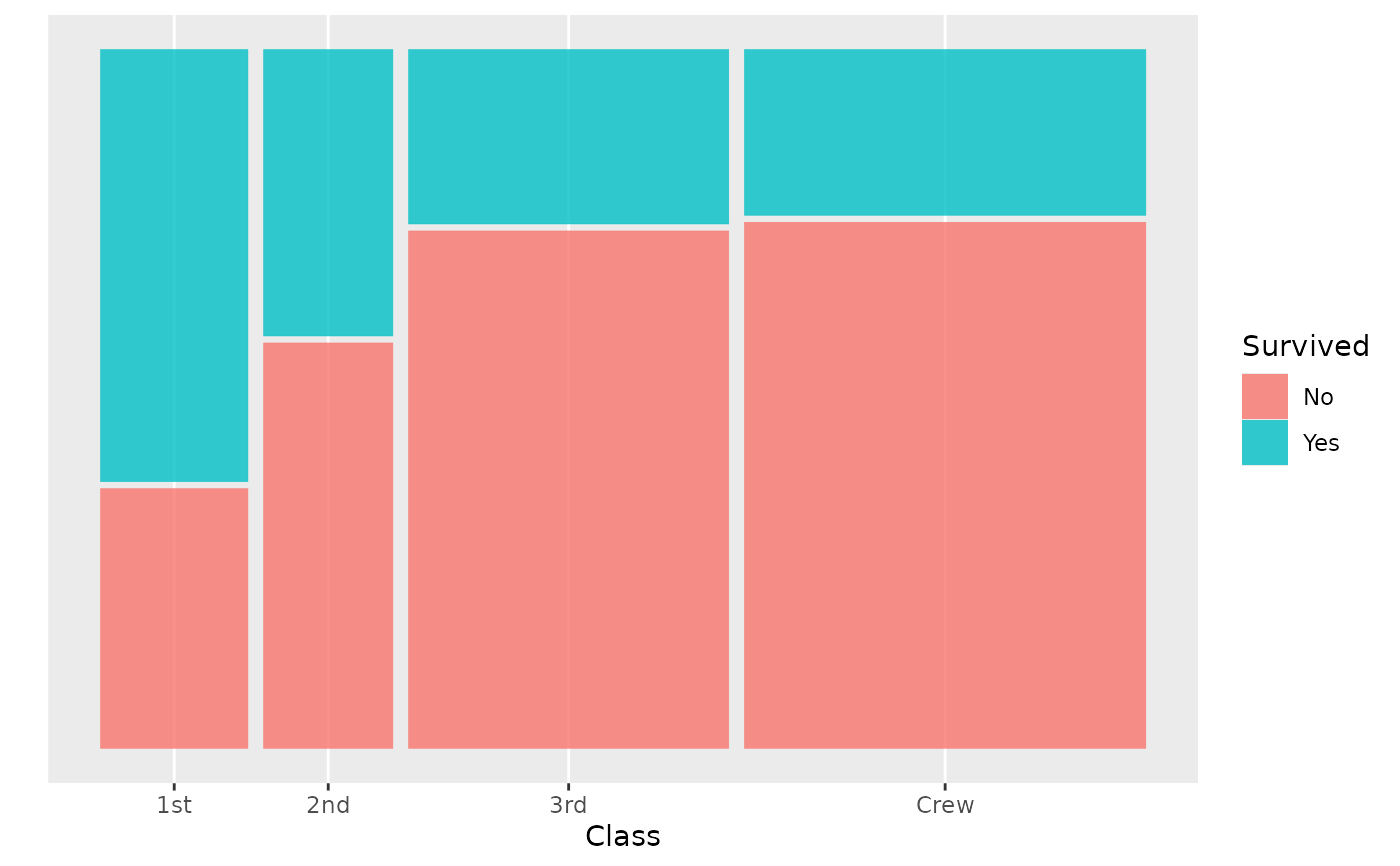 # good practice: use the 'dependent' variable (or most important variable)
# as fill variable
# if there is only one variable inside `product()`,
# `product()` can be omitted
ggplot(data = titanic, aes(x = Class, fill = Survived)) +
geom_mosaic()
# good practice: use the 'dependent' variable (or most important variable)
# as fill variable
# if there is only one variable inside `product()`,
# `product()` can be omitted
ggplot(data = titanic, aes(x = Class, fill = Survived)) +
geom_mosaic()
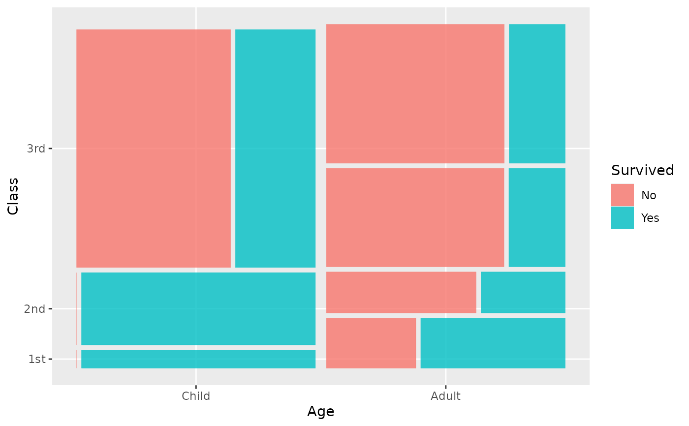
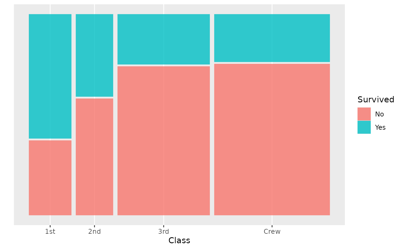 ggplot(data = titanic,
aes(x = product(Class, Age), fill = Survived)) +
geom_mosaic()
ggplot(data = titanic,
aes(x = product(Class, Age), fill = Survived)) +
geom_mosaic()
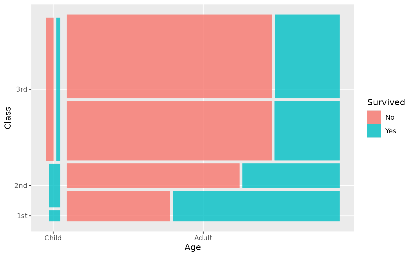 ggplot(data = titanic,
aes(x = product(Class), conds = product(Age), fill = Survived)) +
geom_mosaic()
ggplot(data = titanic,
aes(x = product(Class), conds = product(Age), fill = Survived)) +
geom_mosaic()
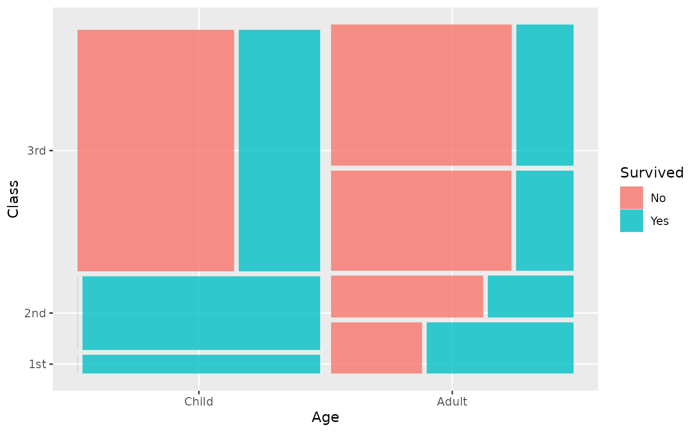 # if there is only one variable inside `product()`,
# `product()` can be omitted
ggplot(data = titanic, aes(x = Class, conds = Age, fill = Survived)) +
geom_mosaic()
# if there is only one variable inside `product()`,
# `product()` can be omitted
ggplot(data = titanic, aes(x = Class, conds = Age, fill = Survived)) +
geom_mosaic()
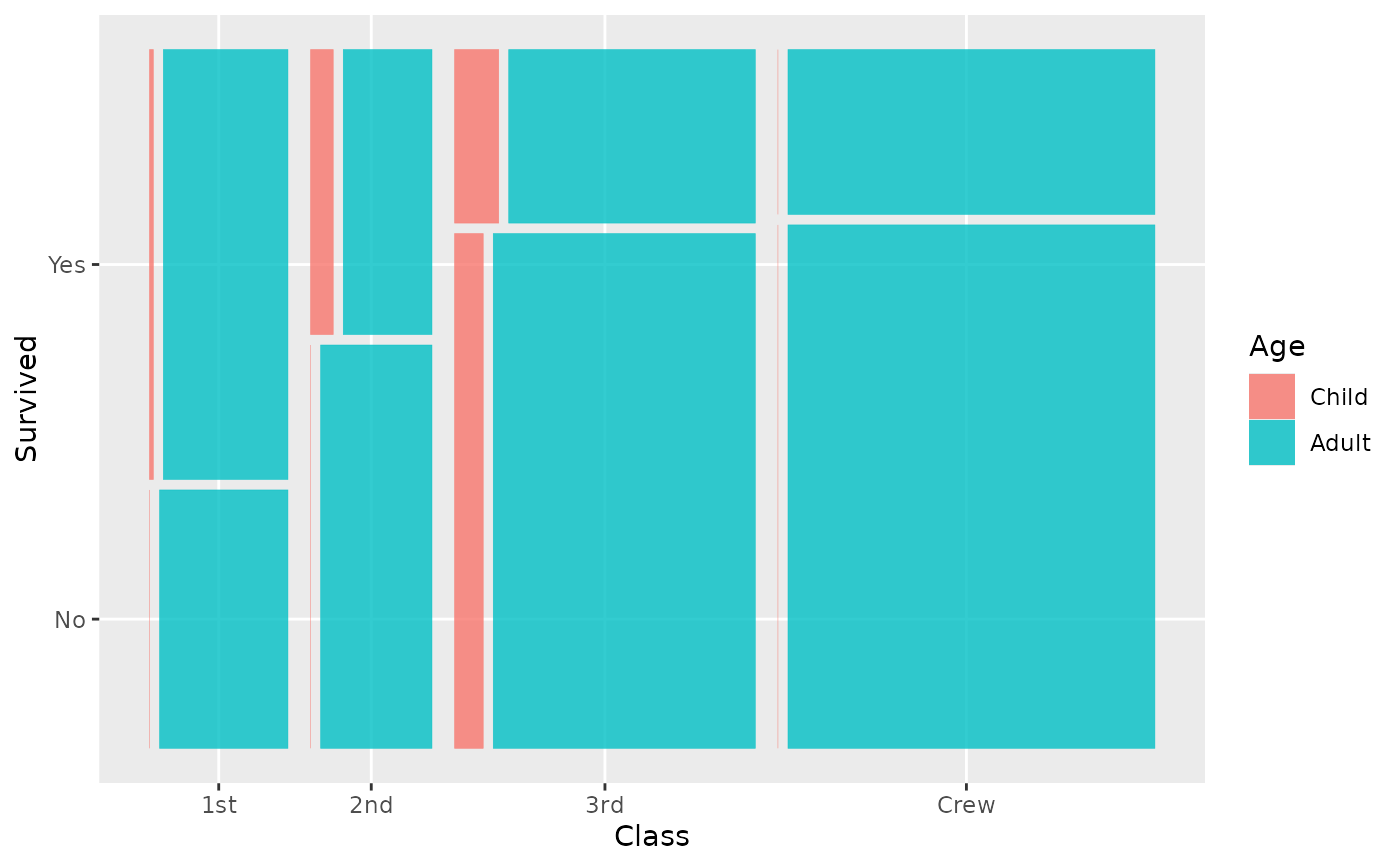
 ggplot(data = titanic,
aes(x = product(Survived, Class), fill = Age)) +
geom_mosaic()
ggplot(data = titanic,
aes(x = product(Survived, Class), fill = Age)) +
geom_mosaic()
 # Variables can be transformed directly inside mosaic aesthetics
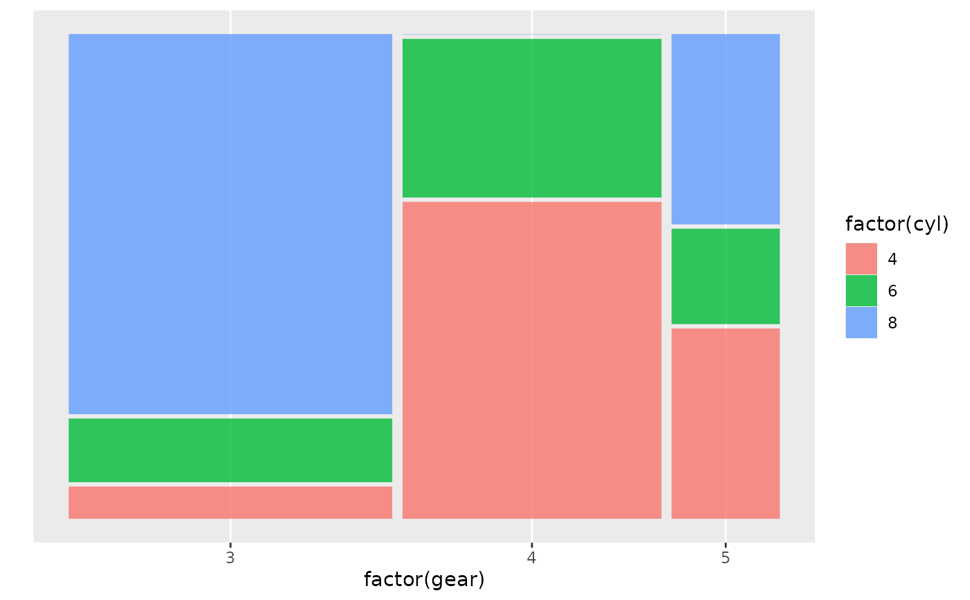
ggplot(data = mtcars,
aes(x = product(factor(gear)), fill = factor(cyl))) +
geom_mosaic()
# Variables can be transformed directly inside mosaic aesthetics
ggplot(data = mtcars,
aes(x = product(factor(gear)), fill = factor(cyl))) +
geom_mosaic()
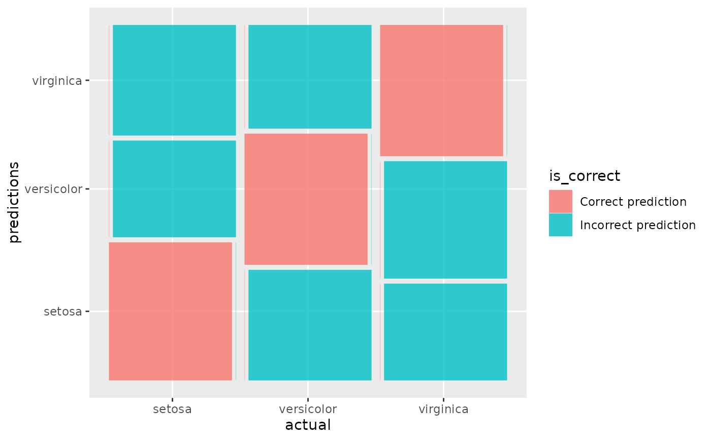
 # A fill-only variable colours and partitions the tiles without appearing on
# a position axis. Reverse the product order to put `actual` on the x axis.
set.seed(19790801)
predictions <- sample(iris$Species)
confusion <- as.data.frame(table(actual = iris$Species, predictions))
confusion$is_correct <- ifelse(
confusion$actual == confusion$predictions,
"Correct prediction", "Incorrect prediction"
)
ggplot(confusion, aes(
weight = Freq,
x = product(predictions, actual),
fill = is_correct
)) +
geom_mosaic()
# A fill-only variable colours and partitions the tiles without appearing on
# a position axis. Reverse the product order to put `actual` on the x axis.
set.seed(19790801)
predictions <- sample(iris$Species)
confusion <- as.data.frame(table(actual = iris$Species, predictions))
confusion$is_correct <- ifelse(
confusion$actual == confusion$predictions,
"Correct prediction", "Incorrect prediction"
)
ggplot(confusion, aes(
weight = Freq,
x = product(predictions, actual),
fill = is_correct
)) +
geom_mosaic()
 # Wrapped in donttest: still runs under R CMD check --run-donttest and is
# exercised by the package's tests to make sure it works.
# \donttest{
data(happy)
ggplot(data = happy, aes(x = product(happy))) +
geom_mosaic(divider = "hbar")
# Wrapped in donttest: still runs under R CMD check --run-donttest and is
# exercised by the package's tests to make sure it works.
# \donttest{
data(happy)
ggplot(data = happy, aes(x = product(happy))) +
geom_mosaic(divider = "hbar")
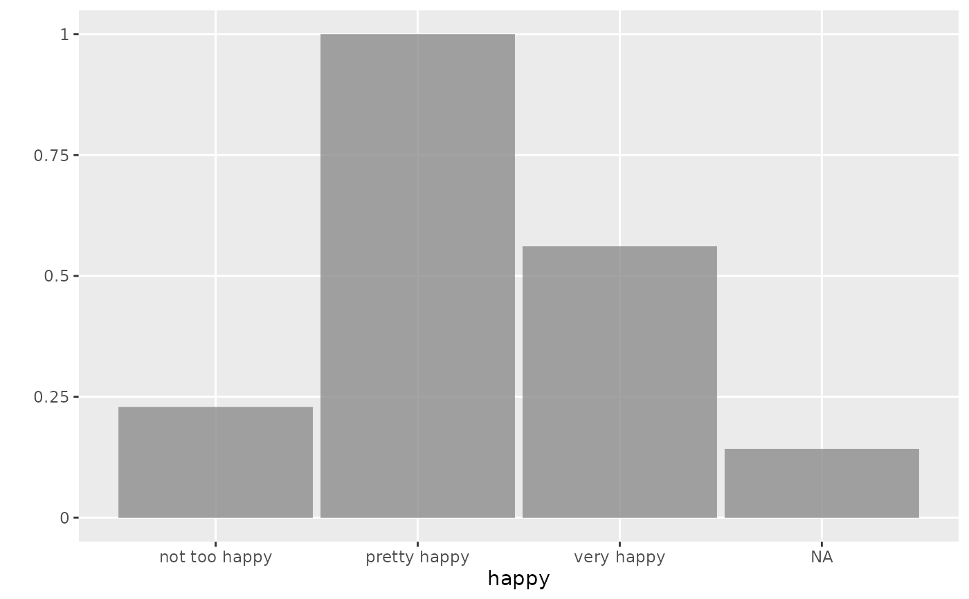 ggplot(data = happy, aes(x = product(happy))) +
geom_mosaic() +
coord_flip()
ggplot(data = happy, aes(x = product(happy))) +
geom_mosaic() +
coord_flip()
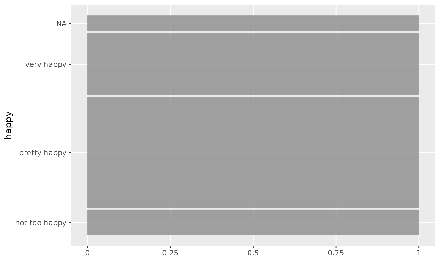 # weighting is important
ggplot(data = happy, aes(weight = wtssall, x = product(happy))) +
geom_mosaic()
# weighting is important
ggplot(data = happy, aes(weight = wtssall, x = product(happy))) +
geom_mosaic()
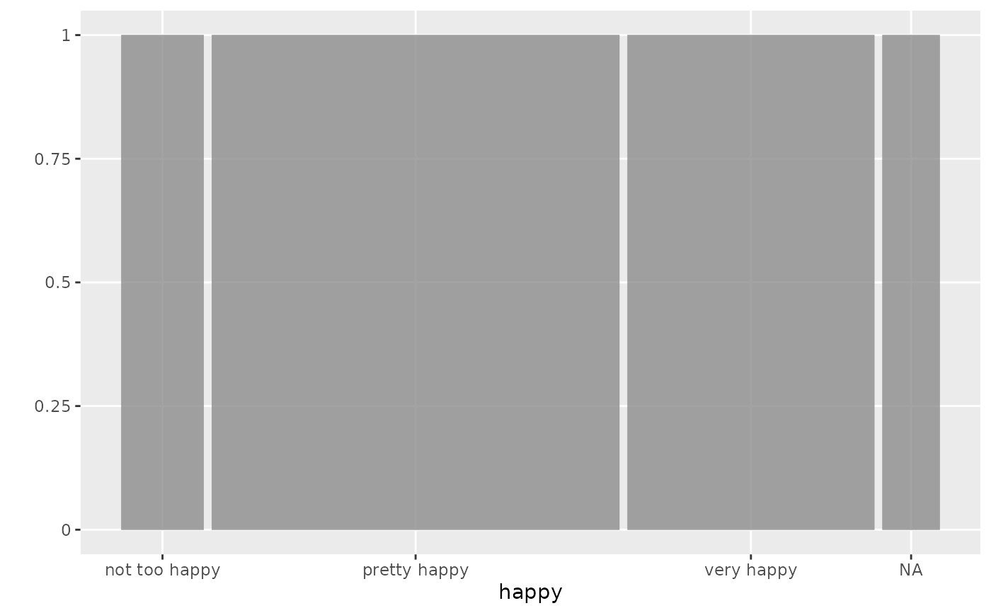 ggplot(data = happy,
aes(weight = wtssall, x = product(health), fill = happy)) +
geom_mosaic() +
theme(axis.text.x=element_text(angle=35))
ggplot(data = happy,
aes(weight = wtssall, x = product(health), fill = happy)) +
geom_mosaic() +
theme(axis.text.x=element_text(angle=35))
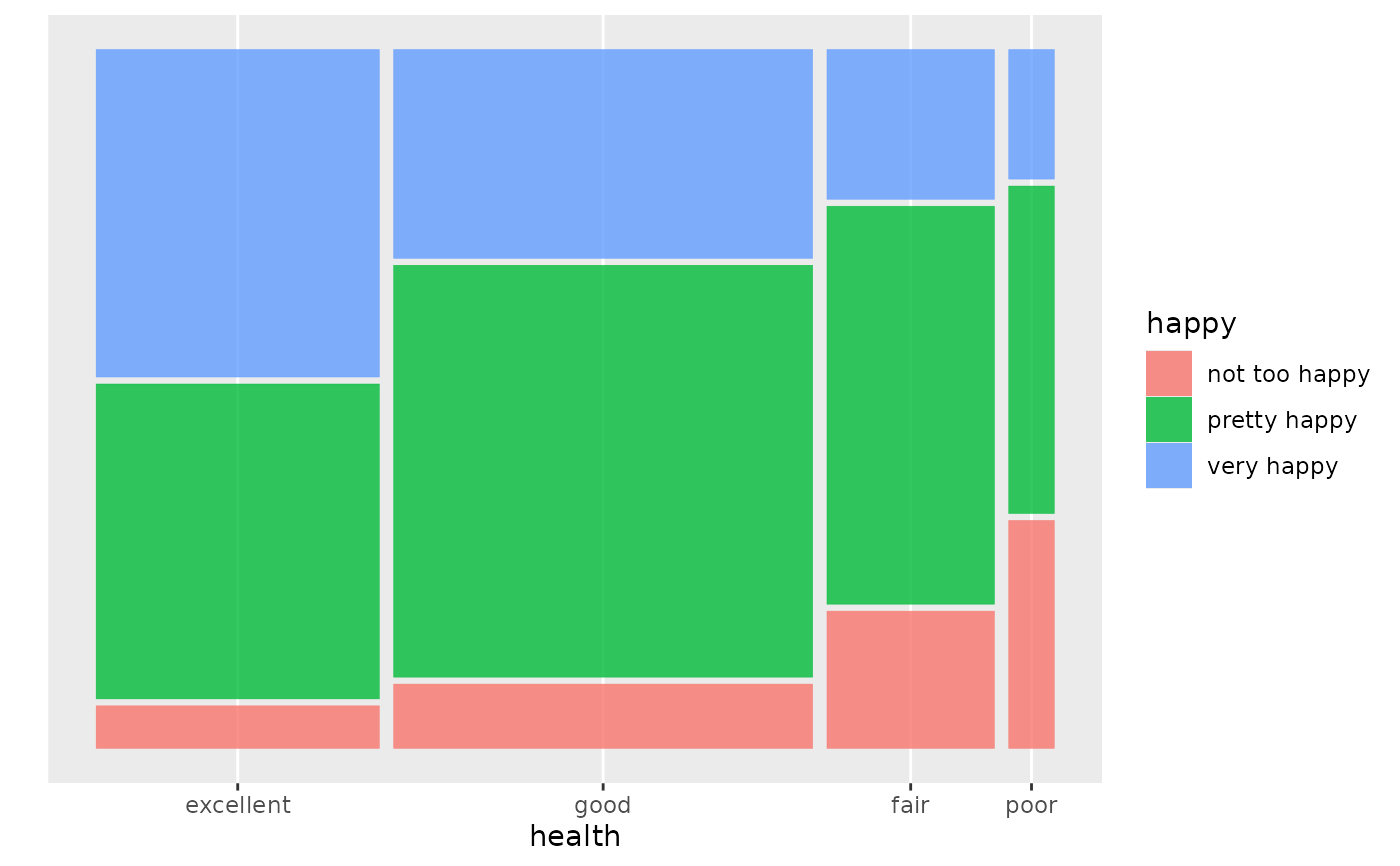
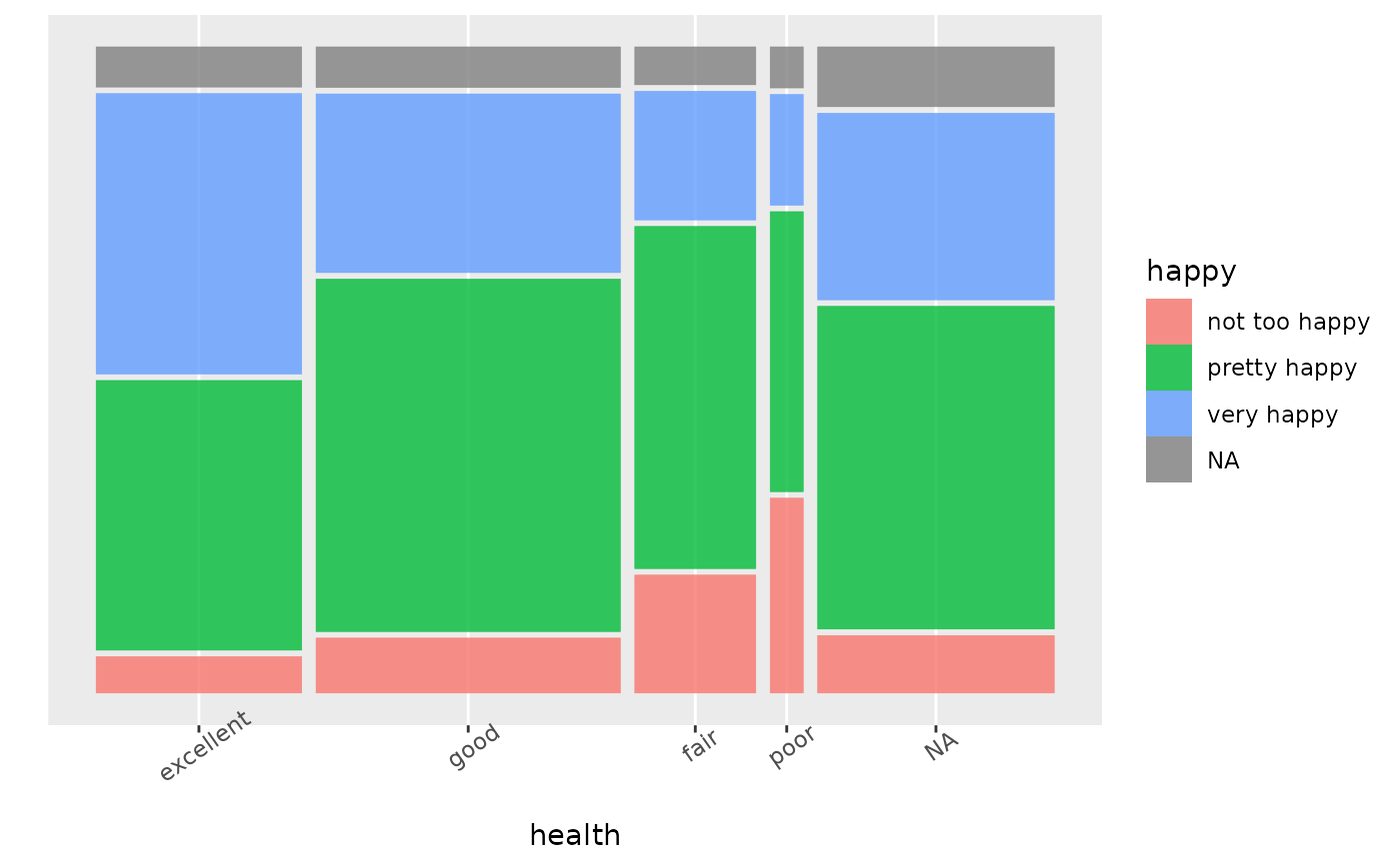 ggplot(data = happy,
aes(weight = wtssall, x = product(health), fill = happy)) +
geom_mosaic(na.rm = TRUE)
ggplot(data = happy,
aes(weight = wtssall, x = product(health), fill = happy)) +
geom_mosaic(na.rm = TRUE)
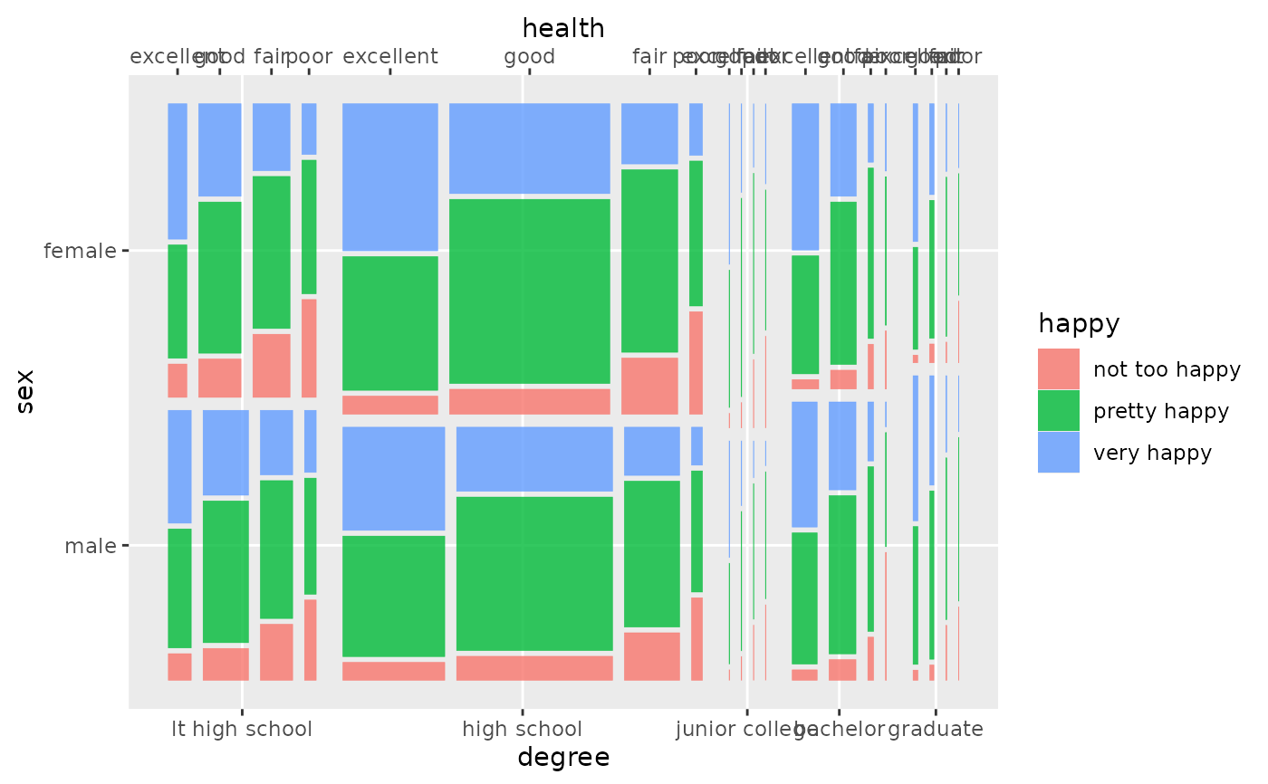
 ggplot(data = happy,
aes(weight = wtssall, x = product(health, sex, degree), fill = happy)) +
geom_mosaic(na.rm = TRUE)
ggplot(data = happy,
aes(weight = wtssall, x = product(health, sex, degree), fill = happy)) +
geom_mosaic(na.rm = TRUE)
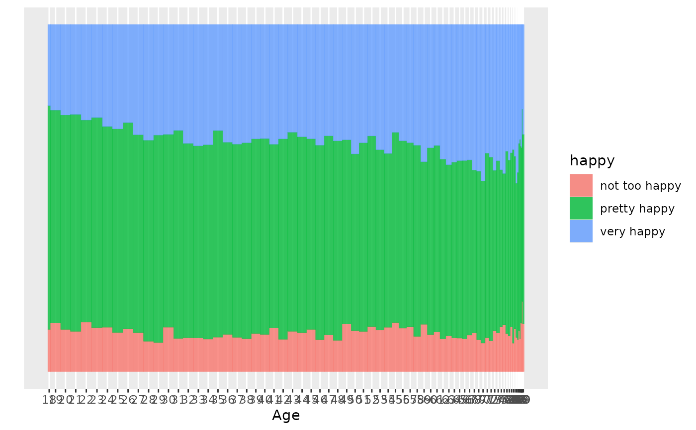
 # here is where a bit more control over the spacing of the bars is helpful:
# set labels manually:
ggplot(data = happy,
aes(weight = wtssall, x = product(age), fill = happy)) +
geom_mosaic(na.rm = TRUE, offset = 0) +
scale_x_productlist("Age", labels=c(17+1:72))
# here is where a bit more control over the spacing of the bars is helpful:
# set labels manually:
ggplot(data = happy,
aes(weight = wtssall, x = product(age), fill = happy)) +
geom_mosaic(na.rm = TRUE, offset = 0) +
scale_x_productlist("Age", labels=c(17+1:72))
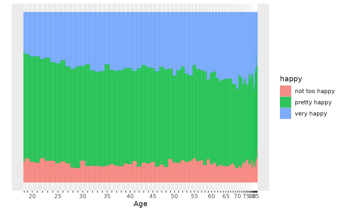
 # thin out labels manually:
labels <- c(17+1:72)
labels[labels %% 5 != 0] <- ""
ggplot(data = happy,
aes(weight = wtssall, x = product(age), fill = happy)) +
geom_mosaic(na.rm = TRUE, offset = 0) +
scale_x_productlist("Age", labels=labels)
# thin out labels manually:
labels <- c(17+1:72)
labels[labels %% 5 != 0] <- ""
ggplot(data = happy,
aes(weight = wtssall, x = product(age), fill = happy)) +
geom_mosaic(na.rm = TRUE, offset = 0) +
scale_x_productlist("Age", labels=labels)
 ggplot(data = happy,
aes(weight = wtssall, x = product(age), fill = happy,
conds = product(sex))) +
geom_mosaic(divider = mosaic("v"), na.rm = TRUE, offset = 0.001) +
scale_x_productlist("Age", labels=labels)
ggplot(data = happy,
aes(weight = wtssall, x = product(age), fill = happy,
conds = product(sex))) +
geom_mosaic(divider = mosaic("v"), na.rm = TRUE, offset = 0.001) +
scale_x_productlist("Age", labels=labels)
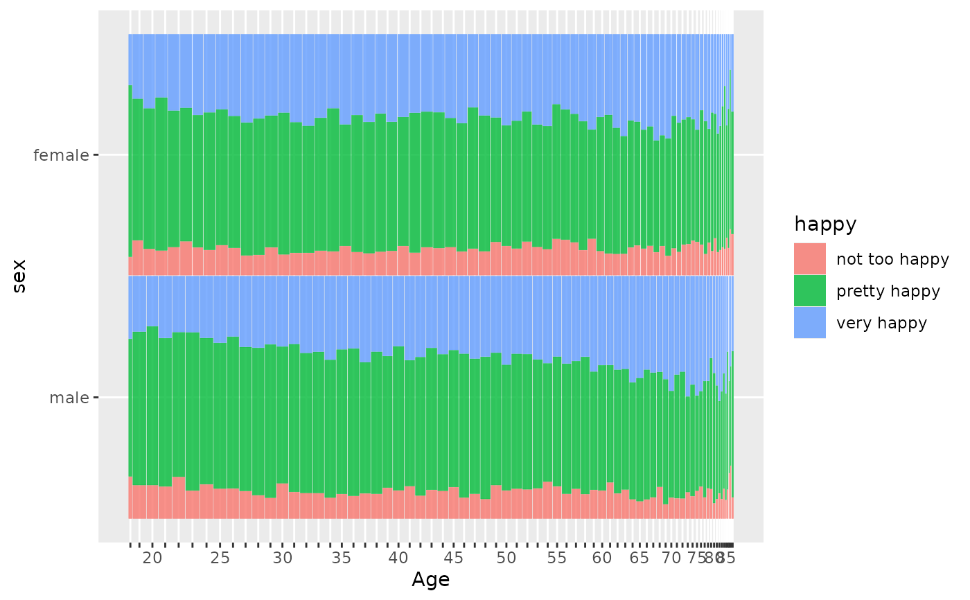 ggplot(data = happy,
aes(weight = wtssall, x = product(age), fill = happy)) +
geom_mosaic(na.rm = TRUE, offset = 0) +
facet_grid(sex~.) +
scale_x_productlist("Age", labels=labels)
ggplot(data = happy,
aes(weight = wtssall, x = product(age), fill = happy)) +
geom_mosaic(na.rm = TRUE, offset = 0) +
facet_grid(sex~.) +
scale_x_productlist("Age", labels=labels)
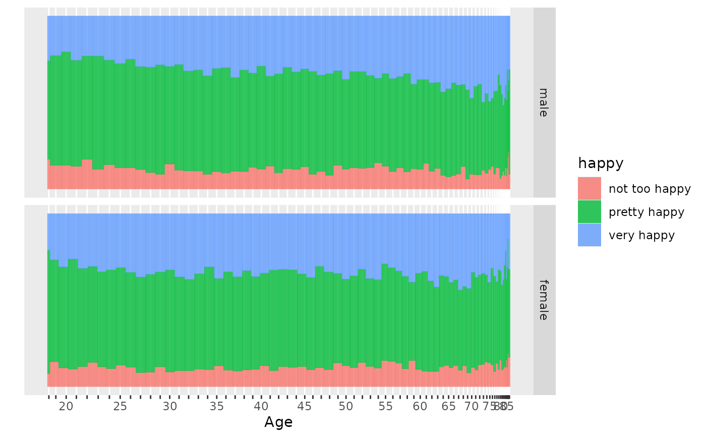 ggplot(data = happy,
aes(weight = wtssall, x = product(happy, finrela, health))) +
geom_mosaic(divider = mosaic("h"))
ggplot(data = happy,
aes(weight = wtssall, x = product(happy, finrela, health))) +
geom_mosaic(divider = mosaic("h"))
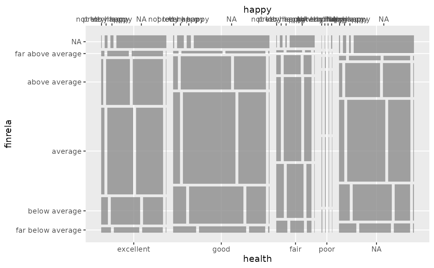 ggplot(data = happy,
aes(weight = wtssall, x = product(happy, finrela, health))) +
geom_mosaic(offset = .005)
ggplot(data = happy,
aes(weight = wtssall, x = product(happy, finrela, health))) +
geom_mosaic(offset = .005)
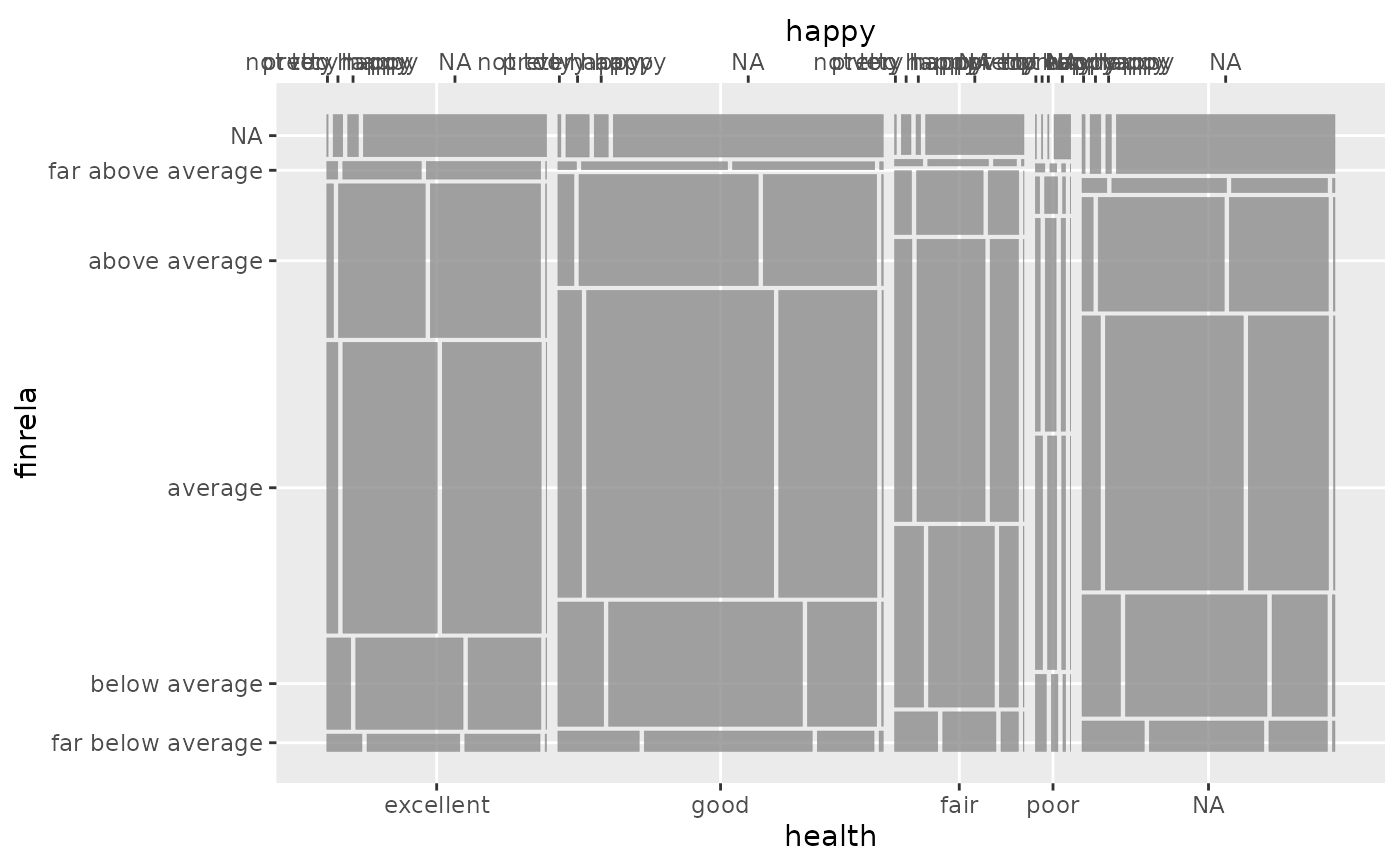 # Spine example
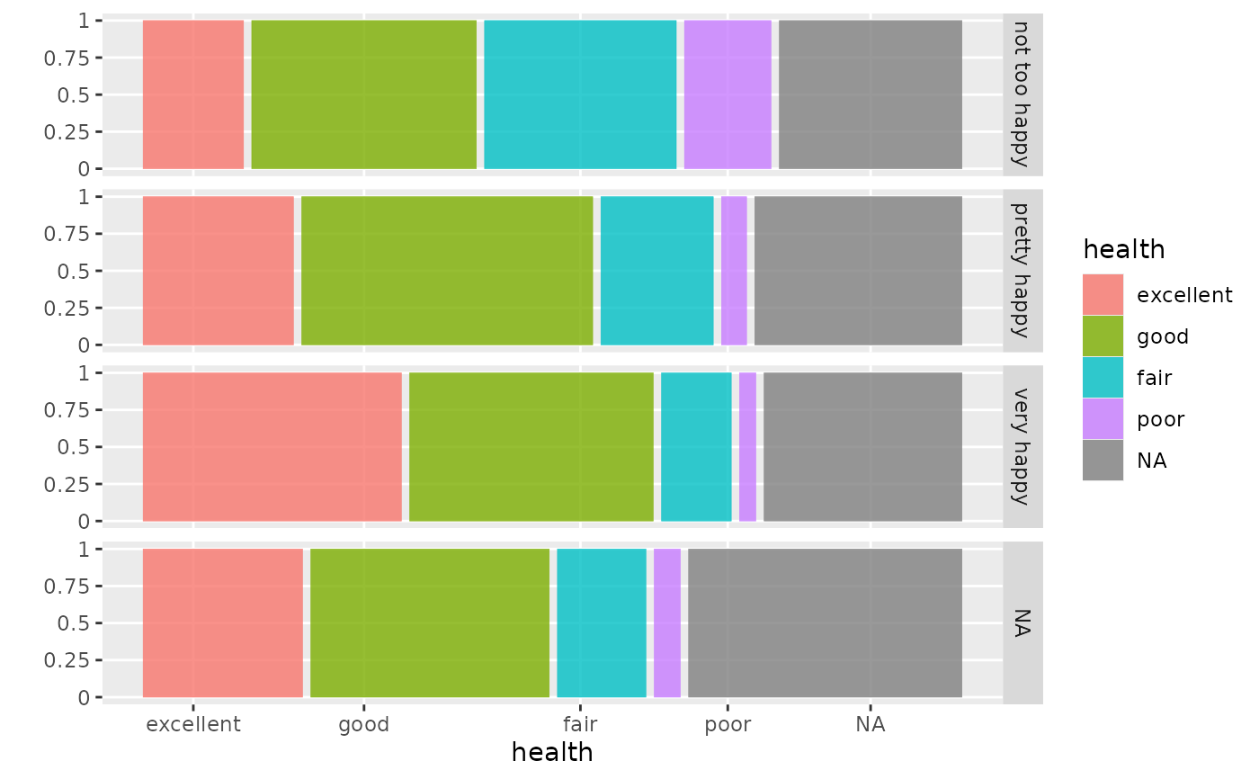
ggplot(data = happy,
aes(weight = wtssall, x = product(health), fill = health)) +
geom_mosaic() +
facet_grid(happy~.)
# Spine example
ggplot(data = happy,
aes(weight = wtssall, x = product(health), fill = health)) +
geom_mosaic() +
facet_grid(happy~.)
 # Residual shading with independence model
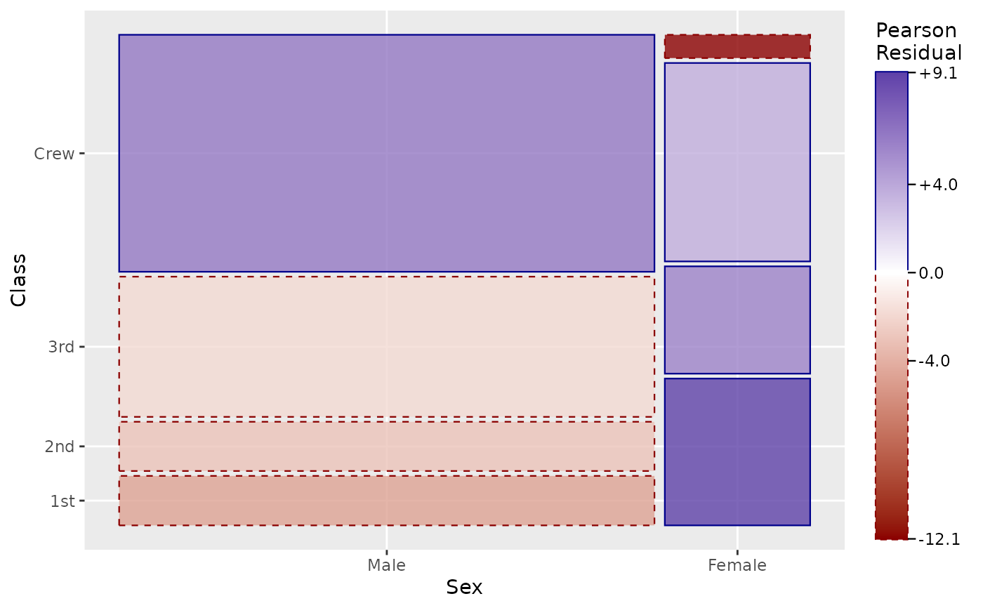
ggplot(data = titanic, aes(x = product(Class, Sex))) +
geom_mosaic(expected = "independence") +
scale_fill_residual()
# Residual shading with independence model
ggplot(data = titanic, aes(x = product(Class, Sex))) +
geom_mosaic(expected = "independence") +
scale_fill_residual()
 # Custom model formula
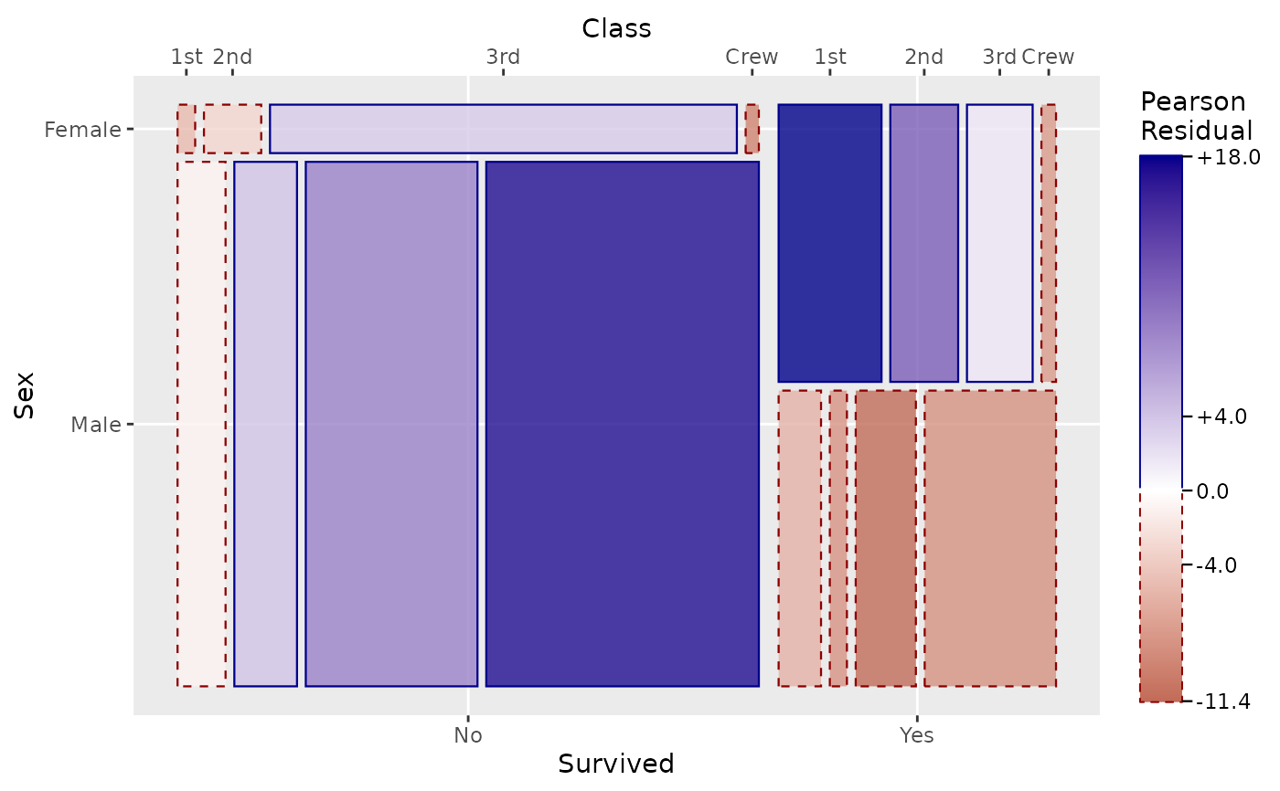
ggplot(data = titanic, aes(x = product(Class, Sex, Survived))) +
geom_mosaic(expected = ~ Class + Sex) +
scale_fill_residual()
# Custom model formula
ggplot(data = titanic, aes(x = product(Class, Sex, Survived))) +
geom_mosaic(expected = ~ Class + Sex) +
scale_fill_residual()
 # } # end of donttest