The Logarithmic Series Distribution

The logarithmic series distribution is a long-tailed distribution introduced by Fisher etal. (1943) in connection with data on the abundance of individuals classified by species.

Usage

dlogseries(x, prob = 0.5, log = FALSE)

plogseries(q, prob = 0.5, lower.tail = TRUE, log.p = FALSE)

qlogseries(p, prob = 0.5, lower.tail = TRUE, log.p = FALSE, max.value = 10000)

rlogseries(n, prob = 0.5)

Arguments

x, q: vector of quantiles representing the number of events.
prob: parameter for the distribution, 0 < prob < 1
log, log.p: logical; if TRUE, probabilities p are given as log(p)
lower.tail: logical; if TRUE (default), probabilities are $P[X \le x]$, otherwise, $P[X > x]$.
p: vector of probabilities
max.value: maximum value returned by qlogseries
n: number of observations for rlogseries

Value

dlogseries gives the density, plogseries gives the cumulative distribution function, qlogseries gives the quantile function, and rlogseries generates random deviates.

Details

These functions provide the density, distribution function, quantile function and random generation for the logarithmic series distribution with parameter prob.

The logarithmic series distribution with prob = $p$ has density $$ p ( x ) = \alpha p^x / x $$ for $x = 1, 2, \dots$, where $\alpha= -1 / \log(1 - p)$ and $0 < p < 1$. % Note that counts x==2 cannot occur.

References

https://en.wikipedia.org/wiki/Logarithmic_distribution

Fisher, R. A. and Corbet, A. S. and Williams, C. B. (1943). The relation between the number of species and the number of individuals Journal of Animal Ecology, 12, 42-58.

Author

Michael Friendly, using original code modified from the gmlss.dist package by Mikis Stasinopoulos.

Examples


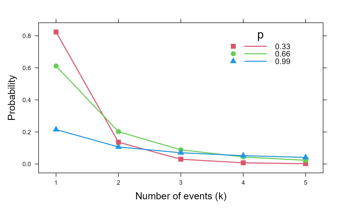
XL <-expand.grid(x=1:5, p=c(0.33, 0.66, 0.99))
lgs.df <- data.frame(XL, prob=dlogseries(XL[,"x"], XL[,"p"]))
lgs.df$p = factor(lgs.df$p)
str(lgs.df)
#> 'data.frame':	15 obs. of  3 variables:
#>  $ x   : int  1 2 3 4 5 1 2 3 4 5 ...
#>  $ p   : Factor w/ 3 levels "0.33","0.66",..: 1 1 1 1 1 2 2 2 2 2 ...
#>  $ prob: num  0.82402 0.13596 0.02991 0.0074 0.00195 ...

require(lattice)
#> Loading required package: lattice
#> 
#> Attaching package: ‘lattice’
#> The following object is masked from ‘package:seriation’:
#> 
#>     panel.lines
#> The following object is masked from ‘package:gnm’:
#> 
#>     barley
mycol <- palette()[2:4]
xyplot( prob ~ x, data=lgs.df, groups=p,
  xlab=list('Number of events (k)', cex=1.25),
  ylab=list('Probability',  cex=1.25),
  type='b', pch=15:17, lwd=2, cex=1.25, col=mycol,
  key = list(
          title = 'p',
          points = list(pch=15:17, col=mycol, cex=1.25),
          lines = list(lwd=2, col=mycol),
          text = list(levels(lgs.df$p)),
          x=0.9, y=0.98, corner=c(x=1, y=1)
          )
  )



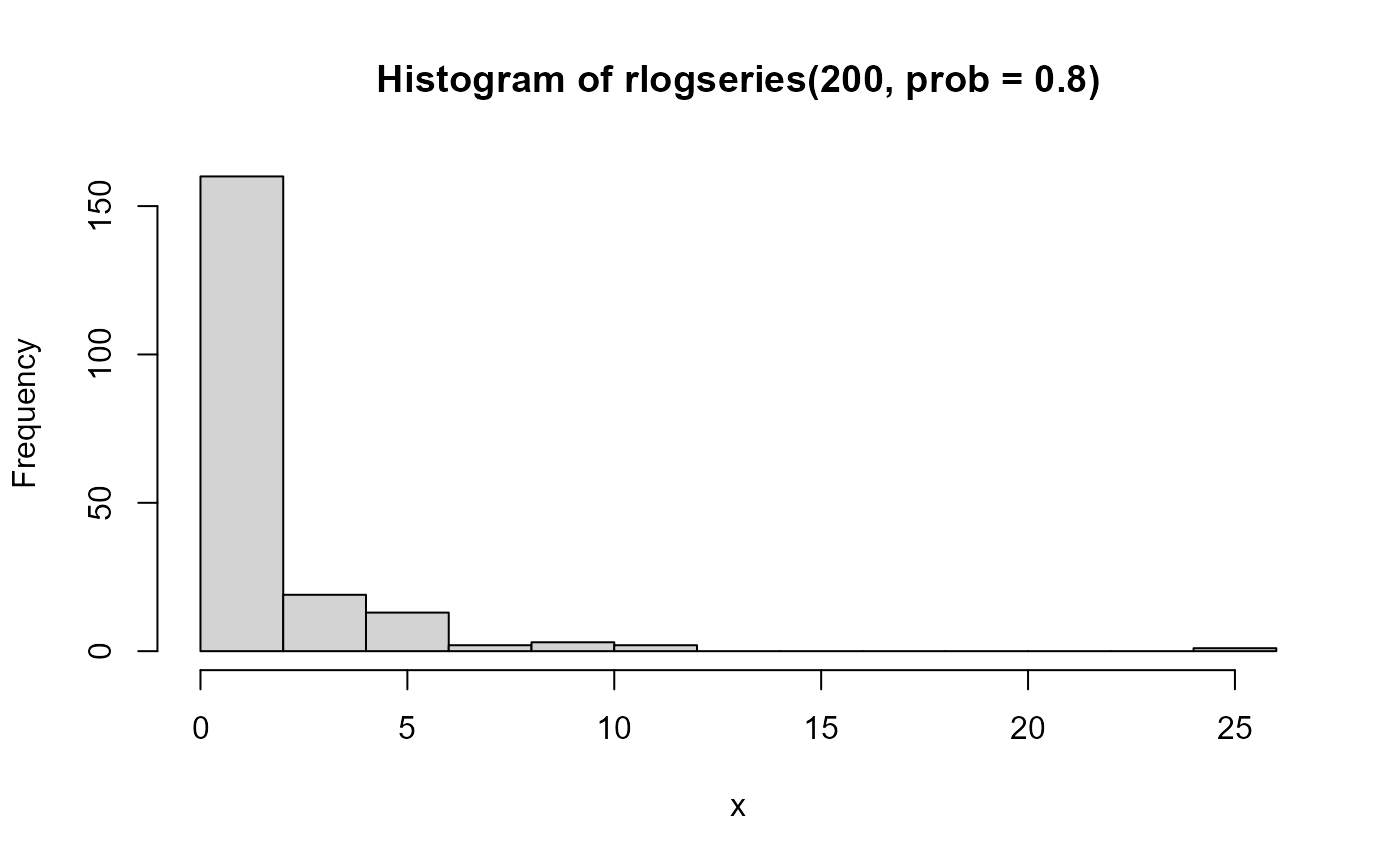
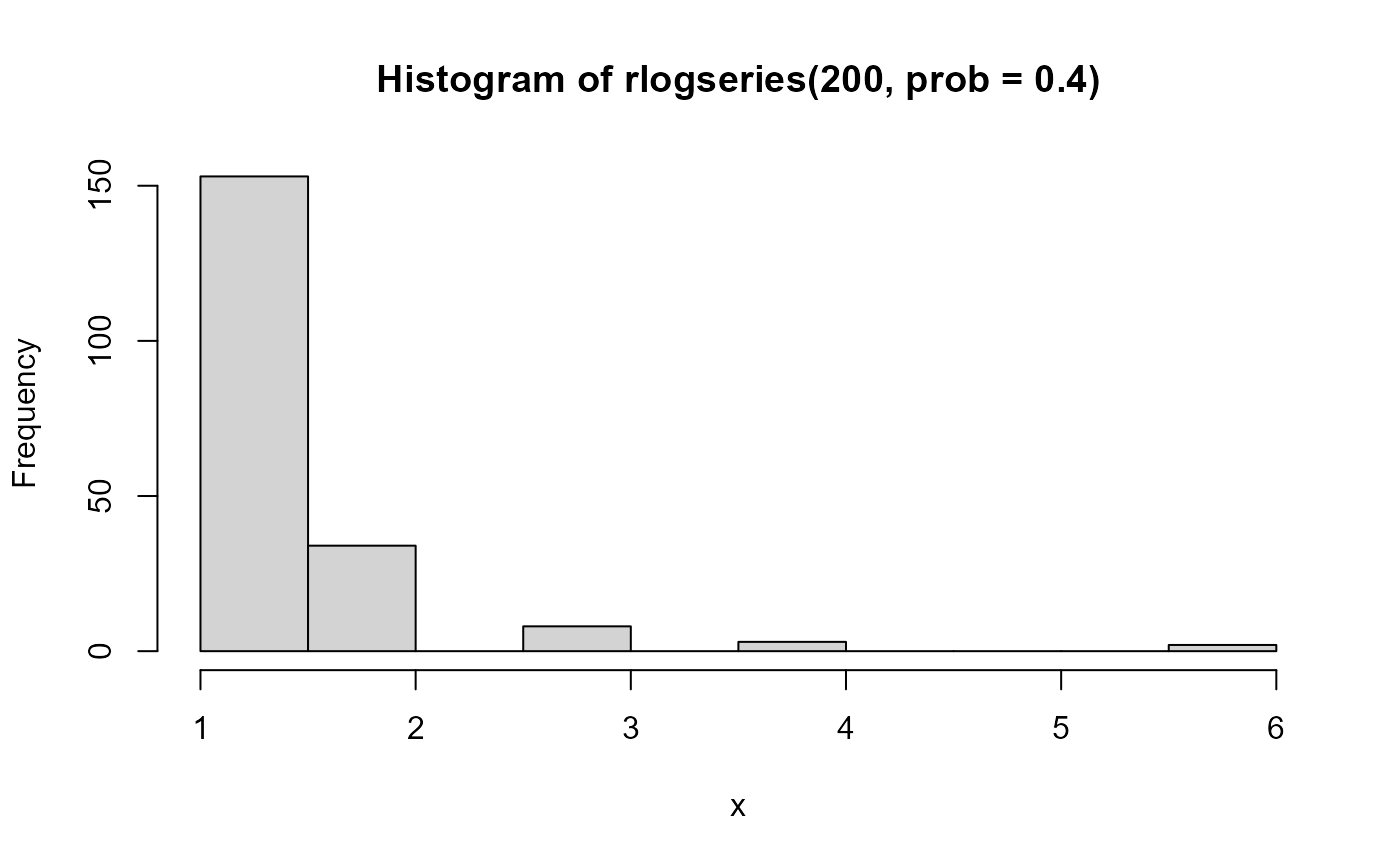
# random numbers
hist(rlogseries(200, prob=.4), xlab='x')

hist(rlogseries(200, prob=.8), xlab='x')