Properties of determinants

Michael Friendly

2024-10-03

The following examples illustrate the basic properties of the determinant of a matrix. We do this first with simple numerical examples and then using geometric diagrams.

Create a 2 x 2 matrix

A <- matrix(c(3, 1, 
              2, 4), nrow=2, byrow=TRUE)
A

##      [,1] [,2]
## [1,]    3    1
## [2,]    2    4

det(A)

## [1] 10

1. Interchange two rows or cols changes the sign: -> -1 * det(A)

det(A[ 2:1, ])

## [1] -10

det(A[, 2:1 ])

## [1] -10

2. transpose -> det (A) unchanged

det( t(A) )

## [1] 10

3. multiply row * k -> k * det(A)

Note that to multiply rows by different constants requires a diagonal matrix on the left.

diag(c(3, 1)) %*% A

##      [,1] [,2]
## [1,]    9    3
## [2,]    2    4

det( diag(c(3, 1))  %*% A)

## [1] 30

4. multiply matrix * k -> k^2 * det(A)

This is because multiplying a matrix by a constant multiplies each row.

det(3 * A)

## [1] 90

3^2 * det(A)

## [1] 90

5. det (A B) -> det(A) * det(B)

The determinant of a product is the product of the determinants. The same holds for any number of terms in a matrix product.

B <- matrix(c(4, 2, 
             3, 5), nrow=2, byrow=TRUE)
B

##      [,1] [,2]
## [1,]    4    2
## [2,]    3    5

det(A %*% B)

## [1] 140

det(A) * det(B)

## [1] 140

6. proportional rows or columns -> det() == 0

Here we just add an additional copy of column 1 of a matrix, so C[,3] == C[,1]. The determinant is 0 because the columns are linearly dependent.

C <- matrix(c(1, 5, 
             2, 6,
             4, 4), nrow=3, byrow=TRUE)
C <- cbind(C, C[,1])
C

##      [,1] [,2] [,3]
## [1,]    1    5    1
## [2,]    2    6    2
## [3,]    4    4    4

det(C)

## [1] 0

7. Add multiple of one row to another -> det unchanged

This is the principle behind one of the elementary row operations.

A[2,] <- A[2,] - 2*A[1,]
det(A)

## [1] 10

8. Geometric interpretation

Many aspects of matrices and vectors have geometric interpretations. For $2 \times 2$ matrices, the determinant is the area of the parallelogram defined by the rows (or columns), plotted in a 2D space. (For $3 \times 3$ matrices, the determinant is the volume of a parallelpiped in 3D space.)

A <- matrix(c(3, 1, 
              2, 4), nrow=2, byrow=TRUE)
A

##      [,1] [,2]
## [1,]    3    1
## [2,]    2    4

det(A)

## [1] 10

The matlib package has some handy functions (vectors()) for drawing geometric diagrams.

library(matlib)
xlim <- c(0,6)
ylim <- c(0,6)
par(mar=c(3,3,1,1)+.1)
plot(xlim, ylim, type="n", xlab="X1", ylab="X2", asp=1)
sum <- A[1,] + A[2,]
# draw the parallelogram determined by the rows of A
polygon( rbind(c(0,0), A[1,], sum, A[2,]), col=rgb(1,0,0,.2))
vectors(A, labels=c("a1", "a2"), pos.lab=c(4,2))
vectors(sum, origin=A[1,], col="gray")
vectors(sum, origin=A[2,], col="gray")
# add some annotations
text(0,6, "det(A) is the area of its row vectors", pos=4)
text(mean(A[,1]), mean(A[,2]), "det(A)", cex=1.25)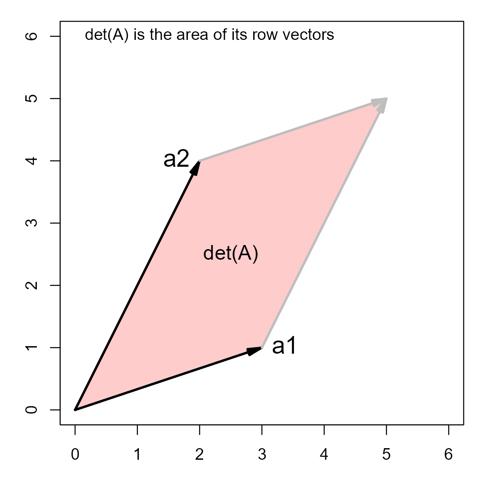

There is a simple visual proof of this fact about determinants but it is easiest to see in the case of a diagonal matrix, where the row vectors are orthogonal, so area is just height x width.

(D <- 2 * diag(2))

##      [,1] [,2]
## [1,]    2    0
## [2,]    0    2

det(D)

## [1] 4

Plot this as before:

par(mar=c(3,3,1,1)+.1)
plot(c(0,2), c(0,2), type="n", xlab="X1", ylab="X2", asp=1)
sum <- D[1,] + D[2,]
polygon( rbind(c(0,0), D[1,], sum, D[2,]), col=rgb(0,1,0,.2))
vectors(D, labels=c("d1", "d2"), pos.lab=c(3,4))
vectors(sum, origin=D[1,], col="gray")
vectors(sum, origin=D[2,], col="gray")
text(mean(D[,1]), mean(D[,2]), "det(D)", cex=1.25)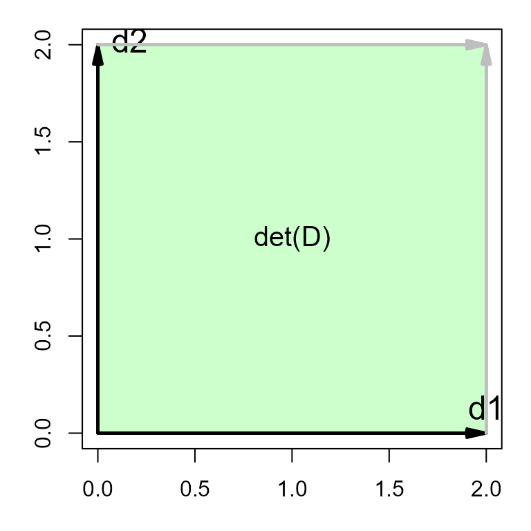

Finally, we can also see why the determinant is zero when the rows or columns are proportional.

(B <- matrix(c(1, 2, 2, 4), 2,2))

##      [,1] [,2]
## [1,]    1    2
## [2,]    2    4

det(B)

## [1] 0

Such vectors are called collinear. They enclose no area.

par(mar=c(3,3,1,1)+.1)
plot(c(0,4), c(0,4), type="n", xlab="X1", ylab="X2", asp=1)
vectors(B, labels=c("b1", "b2"), pos.lab=c(4,2))