Show the code
ggplot(data, aes(x, y)) + geom_point()This is another post in the Making of Vis-MLM series, alongside Quarto Is Not LaTeX, However Hard It Tries (coming soon) and Creating Book Indexes in Quarto. This one is about a smaller, more mechanical problem: once a book has hundreds of code chunks, how do you even find the ones that need attention?
It also touches on the interesting meta-question of How you can use R itself to help with writing about R?.
The title is a small call to mindfulness: in a large book project, it pays to be deliberate about which code you show, how you show it, and whether showing it at all serves the reader. After all, the display of code is part of of the communication goal a book should serve. Chunks should earn their keep!
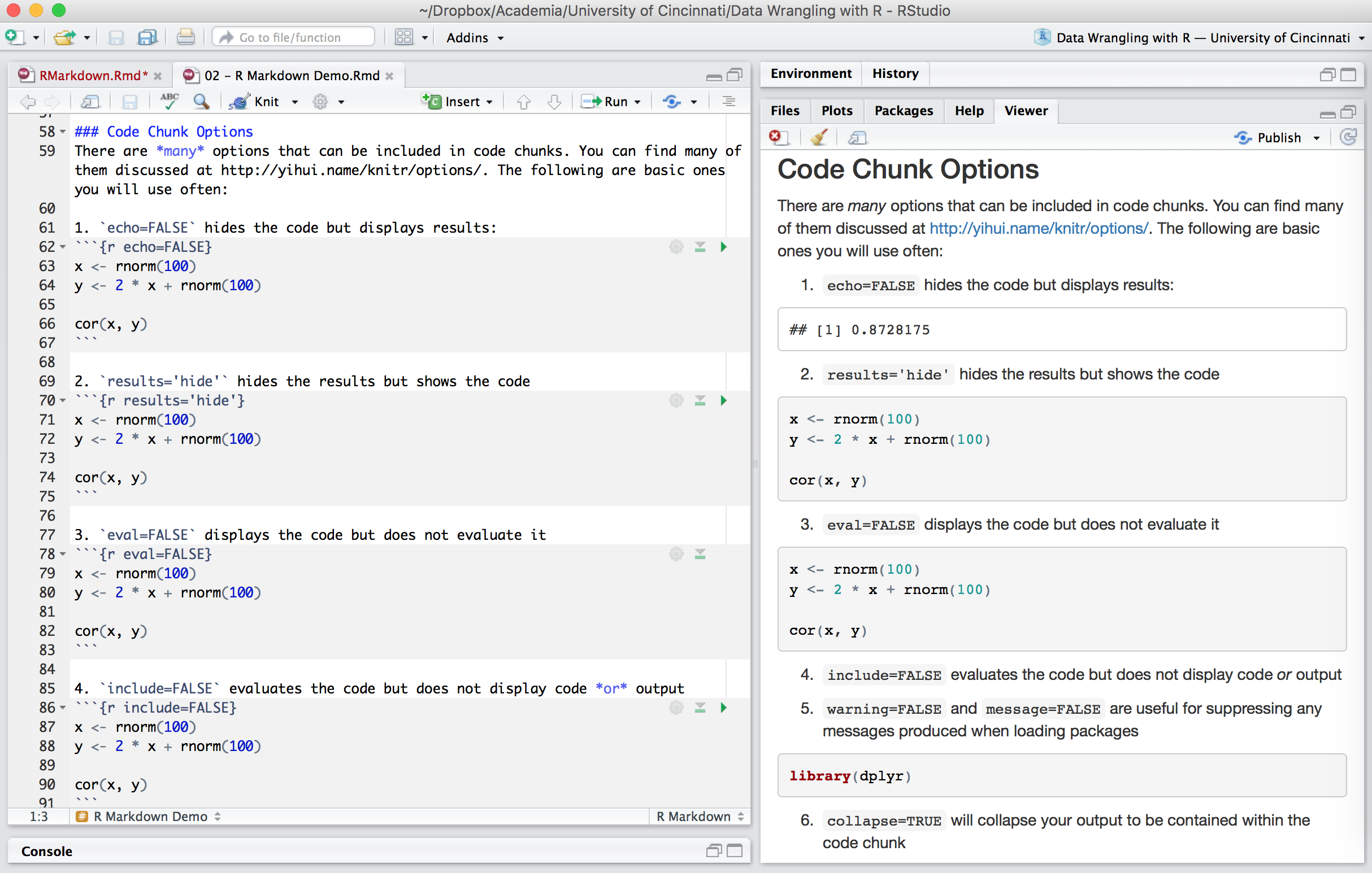
echo, results, eval, and include all shown side by side in RStudio.OK, you’ve written an R-based book with extensive code examples—all analyses and figures are reproducible from source. That’s important! Stemming from Donald Knuth’s (1984) idea of literate programming— the paradigm where computer programs and their explanatory documentation are intertwined into a single, cohesive, reproducible source file— R has evolved for this purpose from Sweave, to RMarkdown, and Quarto. And this aspect of writing about graphical methods and software that does it, is still evolving.
But now, for publication in both online and print form, you ask: is it really necessary to show all that code inline? How does this affect readability, the narrative flow? Or, you see a code block in the PDF that extends outside the shaded box.
A reviewer of my book Visualizing Multivariate Data and Models in R commented that there was too much code on display in the PDF, and that the book could be shortened by folding or hiding some of it. My RA, Gavin Klorfine, also noticed that there were a bunch of code chunks that strayed into the margin. The book contains 281 figures, most generated directly from R code, among 669 chunks throughout the book.
I should mention that I was mindful of these general issues while writing. But the mental work of writing the text—most important—often gave less attention to the details of code display, favoring other work on getting the graphs right.
The question, with this review, became:
Can I make it easier to analyse the properties of all these chunks, in a way that could make editing easier to resolve these and other issues?
One solution to this class of problems, which I implemented by guiding Claude 4.6, involves simply treating your text .qmd files as “data”,
chunks dataset that can be used to analyze and fix such problems.Some aspects of this work may be useful to others, so I describe the problems and solution steps below.
With Quarto, it is easy to fold code in HTML using the YAML chunk option code-fold. In your source .qmd file, it looks like this:
```{r}
#| label: fig-my-plot
#| code-fold: true
#| code-summary: "Show the code"
#| fig-cap: "A scatterplot"
ggplot(data, aes(x, y)) + geom_point()
```
This renders a collapsed “Show the code” button in HTML that the reader can expand at will. Setting code-fold: show makes code visible but still collapsible; code-fold: false forces it always open.
It works like so in HTML:
ggplot(data, aes(x, y)) + geom_point()But code-fold is an HTML-only feature—it has no effect on PDF output, where the code will still appear in full. For print, the relevant option is echo. You can suppress code entirely in PDF while keeping it foldable in HTML with a small knitr trick: put echo = knitr::is_html_output() directly on the chunk header line (not as a #| comment, which won’t work). The header line for the example above becomes:
{r echo=knitr::is_html_output()}
with the other options (label, code-fold, code-summary, fig-cap) staying exactly as before.
Now the code is hidden in PDF and folded-but-available in HTML. The two options work independently: echo=knitr::is_html_output() controls whether code reaches the output at all; code-fold controls how it is presented once it does.
Once you start thinking systematically about code chunks in a large project, other questions come up naturally:
#| label: my-chunk (YAML-style, inside the chunk body), but old-style knitr labels ```{r my-chunk} are still valid. A book that started before Quarto may have a mix. It would be nice to know which files still use the old style in case you want to clean things up.fig-cap set, label starts with fig-), what size are they (fig-width, fig-height, out-width)? This information can be more generally useful in editing the book, standardizing figure sizes and other tasks.eval: false don’t run at all. This was likely designed when writing, but is useful to know when reviewing.The idea is simple: treat your .qmd source files as data and use R to parse them. Each code chunk becomes one tidy row in a data frame, with columns for the attributes mentioned above.
In R, code chunks start with a line matching ```{r and end at the next line that is exactly ```. Everything in between is either a #| YAML option line or code. That structure is regular enough to parse with base-R string tools like grep() and map that over the text using lapply(). No specialized packages needed. (But the stringr package might be a good candidate to simplify the parsing logic here, in another lifetime.)
get_opt() in the snippet below is a small local helper—not from any package. It that scans a vector of #| YAML lines for a given option name and returns its value (or NA if absent):
get_opt <- function(opts, name) {
  pat <- paste0("^#\\|\\s*", name, "\\s*:\\s*(.+)$")
  for (o in opts) {
    m <- regmatches(o, regexec(pat, o))[[1]]
    if (length(m) == 2) return(trimws(m[2]))
  }
  NA_character_
}
Then, we parse chunks that appear in a given chapter .qmd file as follows, returning a list of one item per chunk, with some of it’s options and characteristics:
parse_file_chunks <- function(file) {
  lines  <- readLines(file, warn = FALSE)
  starts <- grep("^```\\{r", lines)          # chunk openings

  lapply(starts, function(s) {
    # find the closing ```
    e <- s + which(grepl("^```\\s*$", lines[(s+1):length(lines)]))[1]

    chunk_lines <- lines[(s+1):e]
    opts <- chunk_lines[grepl("^#\\|", chunk_lines)]   # YAML options
    code <- chunk_lines[!grepl("^#\\|", chunk_lines) &
                        !grepl("^```\\s*$", chunk_lines)]

    list(
      label     = get_opt(opts, "label"),     # #| label: value
      code_fold = get_opt(opts, "code-fold"),
      echo_html = grepl("echo=knitr::is_html_output()", lines[s], fixed=TRUE),
      n_code    = sum(nchar(trimws(code)) > 0)
    )
  })
}
The snippet above is the skeleton. The full script (chunks.R) extends get_opt() calls to cover all the fields listed below—echo_header, echo_opt, code_summary, eval, fig_cap, out_width—plus a few structural ones derived from the file name and chunk position (chapter, line, has_label, old_style, is_fig, n_code_lines). The logic is the same in each case: scan the chunk header or its #| lines with a targeted regex and record what you find (or NA).
The results are then assembled into a data frame by a lapply() simple pass over the active_files, binding the rows together:
do.call(rbind, lapply(active_files, parse_file_chunks))
For a full book project like Vis-MLM, with 19 source files and several active child files, this produces a tidy data frame of 669 chunks with 17 fields:
library(dplyr)
load("data/chunks.RData")
glimpse(chunks)
Rows: 669
Columns: 17
$ chapter <int> 1, 1, 1, 1, 1, 1, 1, 1, 2, 2, 2, 2, 2, 3, 3, 3, 3, 3, 3, …
$ file <chr> "01-Prelude.qmd", "01-Prelude.qmd", "01-Prelude.qmd", "01…
$ line <int> 1, 80, 163, 190, 213, 290, 367, 391, 1, 117, 128, 195, 22…
$ label <chr> NA, NA, "fig-flatland-spheres", "fig-1D-4D", "fig-tessera…
$ has_label <lgl> FALSE, FALSE, TRUE, TRUE, TRUE, TRUE, TRUE, TRUE, FALSE, …
$ old_style <lgl> FALSE, FALSE, FALSE, FALSE, FALSE, FALSE, FALSE, FALSE, F…
$ is_fig <lgl> FALSE, FALSE, TRUE, TRUE, TRUE, FALSE, TRUE, TRUE, FALSE,…
$ echo_html <lgl> FALSE, FALSE, FALSE, FALSE, FALSE, FALSE, FALSE, FALSE, F…
$ echo_header <chr> NA, NA, NA, NA, NA, NA, "-1", NA, NA, NA, NA, NA, "FALSE"…
$ echo_opt <chr> NA, "false", "false", "false", "false", NA, NA, "false", …
$ code_fold <chr> NA, NA, NA, NA, NA, "true", "false", NA, NA, NA, NA, NA, …
$ code_summary <lgl> FALSE, FALSE, FALSE, FALSE, FALSE, TRUE, FALSE, FALSE, FA…
$ eval <chr> NA, NA, NA, NA, NA, "false", NA, NA, NA, NA, NA, NA, NA, …
$ fig_cap <lgl> FALSE, FALSE, TRUE, TRUE, TRUE, TRUE, TRUE, TRUE, FALSE, …
$ out_width <chr> NA, "\"100%\"", "\"90%\"", "\"90%\"", "\"100%\"", NA, "\"…
$ n_code_lines <int> 2, 1, 1, 1, 1, 21, 7, 1, 2, 1, 1, 1, 2, 2, 4, 2, 14, 1, 1…
$ fold_status <chr> "neither", "neither", "neither", "neither", "neither", "n…The fields captured into the chunks database by our script include: chapter, file, line, label, has_label, old_style, is_fig, echo_html, echo_header, echo_opt, code_fold, code_summary, eval, fig_cap, out_width, n_code_lines, and a derived fold_status.
The important point is that you can adapt this script to record any aspects of chunks you want to monitor, analyze, or act on. Your chunks can now work for you.
fold_status fieldThe key derived field is fold_status, which combines code_fold and echo_html into a single summary:
Value (fold_status) |
Meaning |
|---|---|
"both" |
echo_html + code-fold: true—fully folded |
"fold-only" |
code-fold: true but no echo_html—HTML folds, code still in PDF |
"echo-only" |
echo_html but no code-fold—PDF hidden, but code visible in HTML |
"fold-show" |
code-fold: show—always shown, but collapsible |
"fold-false" |
code-fold: false—explicitly kept visible |
"no-eval" |
eval: false—chunk doesn’t run |
"neither" |
No fold treatment at all |
For the Vis-MLM book, the breakdown across 281 figure chunks is:
chunks |>
  filter(is_fig) |>
  count(fold_status, sort = TRUE)
fold_status n
1 neither 227
2 fold-only 19
3 fold-show 15
4 both 14
5 fold-false 3
6 no-eval 3Reading that: neither (227) are potential targets for future folding; fold-only (19) are folded in HTML but code still appears in PDF — incomplete; both (14) are fully folded (Gavin’s audit, this round). The rest (fold-show, fold-false, no-eval) are chunks where the current treatment is intentional rather than an oversight.
The 19 fold-only figure chunks are a useful finding in themselves: they were folded in HTML (probably added before the book targeted PDF), but code still appears in the printed version. Those were candidates for a follow-up editing pass.
With chunks.RData in hand, a few lines of R answer questions that would otherwise require manually scanning thousands of lines of source. Here are just a couple of examples of things I tried:
Which figure chunks still need folding treatment?
Here are longest few (of 227) — the highest-payoff targets for folding. Line numbers help to find them in the chapter files.
chunks |>
  filter(is_fig, fold_status == "neither") |>
  select(chapter, file, line, label, n_code_lines) |>
  slice_max(n_code_lines, n = 8)
chapter file line label n_code_lines
1 11 11-mlm-review.qmd 1456 fig-plastic-ggline 27
2 10 10-hotelling.qmd 401 fig-mathscore-HE-overlay 26
3 5 05-pca-biplot.qmd 842 fig-crime-vectors 22
4 9 09-collinearity-ridge.qmd 698 fig-cars-collin-biplot 22
5 9 09-collinearity-ridge.qmd 851 fig-collin-centering 21
6 14 14-infl-robust.qmd 589 fig-peng-robmlm-plot 20
7 21 21-discrim.qmd 384 fig-peng-new-data 19
8 21 21-discrim.qmd 475 fig-peng-new-discrim2 19
9 21 21-discrim.qmd 648 fig-peng-regions 19How many old-style chunk labels remain?
There’s a lot! I could write a script to fix these if I wanted, but it would have to guess at meaningful chunk labels.
sum(chunks$old_style, na.rm = TRUE)[1] 235I can also ask a question of the book text regarding the relative number of displayed code lines in relation to the number of figures produced in a chapter:
chunks |>
  filter(is_fig, fold_status == "neither") |>
  group_by(chapter, file) |>
  summarise(total_lines = sum(n_code_lines), n_figs = n()) |>
  arrange(desc(total_lines))
# A tibble: 19 × 4
# Groups: chapter [16]
chapter file total_lines n_figs
<int> <chr> <int> <int>
1 5 05-pca-biplot.qmd 168 36
2 12 12-mlm-viz.qmd 168 25
3 4 04-multivariate_plots.qmd 157 27
4 7 07-linear_models-plots.qmd 138 24
5 11 11-mlm-review.qmd 107 17
6 10 10-hotelling.qmd 98 9
7 9 09-collinearity-ridge.qmd 88 15
8 21 21-discrim.qmd 79 7
9 15 15-case-studies.qmd 66 10
10 14 14-infl-robust.qmd 57 8
11 13 13-eqcov.qmd 42 7
12 4 child/04-network.qmd 25 5
13 3 03-getting_started.qmd 24 6
14 6 06-linear_models.qmd 21 3
15 4 child/04-grand-tour.qmd 14 11
16 8 08-lin-mod-topics.qmd 13 6
17 1 01-Prelude.qmd 4 4
18 6 child/06-linear-combinations.qmd 4 4
19 2 02-intro.qmd 3 3From this, the four chapters that are most heavy on my data visualization methods stand out, as they should. Note here that a few child/ documents, included via the knitr option child = are captured in the process.
Gavin’s reviewed the code shown in the HTML and PDF versions for possible folding. His review came back as an .Rmd file with each chunk he flagged marked like ***Label: fig-xxx***. Some of these looked like this:
# Chapter 1: Warm-up Exercises
***Label: fig-diabetes1***
- The narrative here is what the figure shows as opposed to its creation in R

# Chapter 3: Getting Started
***Label: fig-davis-reg1***
- The narrative here is what the figure shows as opposed to its creation in R
***Label: fig-davis-reg2***
- The text describing the reversing of the `x` and `y` axes may be sufficient
 ...
Rather than checking each one by hand against the book source, the script annotate-audit.R looks up every flagged label in chunks and appends its fold_status right there in the review document:
lookup <- with(chunks, setNames(fold_status, label))

pat <- "^(\\*\\*\\*Label: ([^*]+)\\*\\*\\*)(.*)"

for (i in seq_along(lines)) {
  m <- regmatches(lines[i], regexec(pat, lines[i]))[[1]]
  if (length(m) == 0) next

  label  <- trimws(m[3])
  status <- if (label %in% names(lookup)) lookup[[label]] else "NOT IN DATASET"
  lines[i] <- paste0(m[2], " [FOLDED: ", status, "]", m[4])
}
A line like ***Label: fig-scatter*** in the review becomes ***Label: fig-scatter*** [FOLDED: fold-only]—turning a manual cross-check into a one-line lookup, with no risk of missing a flagged chunk or misreading its status.
For the most part in writing, I tried to be careful about formatting code for readability. But not always. Rather than reviewing every such chunk manually, there was a fix within the Quarto rendering process.
Code lines that overflow the shaded box in a PDF book have a root cause in LaTeX geometry: the available width is set by \textwidth (determined by the document class and trim size) minus the padding of the code-block environment. For this book (krantz2 class, letterpaper, 10 pt, Fira Mono in a tcolorbox) the safe limit works out to roughly 65 characters per line, well below R’s default options(width = 80).
Two fixes operate at different levels:
fvextra (a fancyvrb extension) and setting breaklines=true on the Highlighting environment makes any line that exceeds the box width wrap automatically, with a small continuation symbol—no source edits required. Plain fancyvrb does not support breaklines; fvextra must be loaded first (after fancyvrb, which Pandoc loads in its generated preamble):\usepackage{fvextra}
\RecustomVerbatimEnvironment{Highlighting}{Verbatim} %
{commandchars=\\\{\},breaklines=true,breakanywhere=true}breaklines=true wraps at spaces; breakanywhere=true additionally breaks mid-token for long strings or identifiers with no internal spaces.
issues/wide-code.R extends the chunk-scanning approach to measure line widths. It expands tabs with the same tabstop = 4 rule that knitr uses, then flags every code line exceeding the limit—but only in chunks that are actually visible in the PDF (skipping echo=knitr::is_html_output(), echo=FALSE, and #| echo: false chunks). The output gives file, line number, chunk label, width, and a text snippet so each case can be located and fixed directly.Once chunks.RData was ready and Gavin’s annotated audit came back, implementing the changes was mechanical. He flagged 15 chunks as candidates for folding across all 19 chapter files (Chs. 1–21 of the book). Fourteen got the two-step treatment—echo=knitr::is_html_output() on the header line, #| code-fold: true and #| code-summary: "Show the code" in the body. The fifteenth, ggally-smooth-fns, was a two-line exploratory listing that didn’t belong as a chunk at all; it was removed and its content folded into surrounding prose.
Four chunks Gavin reviewed were explicitly kept visible. These were places where showing the code is the point—the first figure in Ch. 1 where seeing the ggplot() call is half the lesson, or a reference figure the surrounding text explains line by line.
Before Gavin’s pass, about 30 figure chunks already had code-fold: true from earlier editing, and those show up in the data as fold_status == "fold-only" (19 in the final count): HTML folds them, but code still appears in the printed PDF—an artifact of being folded before the echo_html trick was settled. Gavin’s 14 additions hit the "both" column: hidden in PDF, foldable in HTML.
The remaining 227 figure chunks with fold_status == "neither" are what they look like: simply displayed. This is mostly a communication choice— one aspect of the _Vis-MLM` project is to describe how a given graph was constructed, so the reader could use that method with their own data. I also tried to describe this process step-by-step, so the code for a given graph is often distributed across several chunks. In addition, I also matched the R figures in the book to the corresponding R source files in my project tree, and provide an online appendix of R code.
This approach to writing about R is an example of Chairman Mao’s Dictum: Theory into Practice. It also reflects John W. Tukey’s observation,
The practical power of a statistical test is the product of its’ statistical power and the probability of use. — John W. Tukey (1959), A Quick, Compact, Two Sample Test to Duckworth’s Specifications
But if I ever want to revisit this problem, the database makes it trivial to sort by n_code_lines and find the highest-payoff targets for a follow-up pass. That list exists. It’s just waiting for a rainy afternoon; or, my editor asking if I can trim a few more pages.
My first guess was xfun, Yihui Xie’s grab-bag of utilities behind knitr. But it’s really just a collection of general-purpose file/string helpers (xfun::read_utf8(), xfun::proj_root(), and the like), not a chunk parser. knitr itself comes closer: after a document has been knitted, knitr::knit_code$get() returns every chunk’s code and options from that run. But that only exists after you’ve knitted the whole thing, whereas the point here was to inspect chunks in the “wild”, before running anything.
The package that actually does this job properly is parsermd (by Colin Rundel). parse_rmd() turns a .Rmd/.qmd file into a proper abstract syntax tree (AST)—a tree that mirrors the document’s structure (headings nesting sections, chunks and prose as ordered nodes within them) rather than a flat wall of text—and as_tibble() flattens it to one row per node, with chunk label, engine, and a parsed options list (old-style header args and new-style #| YAML alike) as columns.
A small .qmd fragment like this:
## Introduction

Some introductory text.


::: {.cell}

:::


## Analysis

Here we fit a model.


::: {.cell}

```{.r .cell-code  code-fold="true"}
ggplot(data, aes(x, y)) + geom_point()
```
:::
produces an AST whose structure looks roughly like:
Document
├── Section [h2]: "Introduction"
│   ├── Prose: "Some introductory text."
│   └── Chunk [r, label="setup"]
│           options: {echo: false}
└── Section [h2]: "Analysis"
    ├── Prose: "Here we fit a model."
    └── Chunk [r, label="fig-scatter"]
            options: {fig-cap: "A scatterplot", code-fold: true}
as_tibble() then flattens this to one row per node, making it straightforward to filter for chunks, inspect options, or join against other metadata.
I tried parse_rmd() against a Vis-MLM chapter, it picked up echo=knitr::is_html_output(), code.fold, and even a computed fig.cap expression without complaint. Had I found it first, parsermd would have replaced most of chunks.R’s parsing logic outright, leaving just the project-specific rollup (the fold_status derivation and the auditing queries) to write myself. I found out about it only after the fact, which is itself a small lesson in searching CRAN before writing many lines of regex— not a fun prospect because R’s escaping mechanism means doubling \ characters, which are the heart of a regular expression.
For completeness, the command line tool quarto inspect, was not the answer: it reports document/project-level metadata (formats, engines, extensions), but there is nothing per-chunk.
For a large Quarto/knitr book project, treating code chunks as data pays off quickly. The parsing logic is relatively straightforward—chunks have a regular open/close structure and #| chunkl options are easy to extract. The resulting data frame supports systematic auditing, reviewer cross-checks, and bulk edits that would be tedious to do by hand.
The full script (chunks.R) is available as a GitHub gist. Adapt the active_files list and the child_files vector to your own project structure, and you should be able to build a similar database in a few minutes. Happy Chunk Minding!