Chemical composition of three cultivars of wine

These data are the results of a chemical analysis of wines grown in the same region in Italy but derived from three different cultivars. The analysis determined the quantities of 13 constituents found in each of the three types of wines.

Format

A data frame with 178 observations on the following 14 variables.

Cultivar: a factor with levels barolo grignolino barbera
Alcohol: a numeric vector
MalicAcid: a numeric vector
Ash: a numeric vector
AlcAsh: a numeric vector, Alkalinity of ash
Mg: a numeric vector, Magnesium
Phenols: a numeric vector, Total phenols
Flav: a numeric vector, Flavanoids
NonFlavPhenols: a numeric vector
Proa: a numeric vector, Proanthocyanins
Color: a numeric vector, color intensity
Hue: a numeric vector
OD: a numeric vector, OD280/OD315 of diluted wines
Proline: a numeric vector

Source

This data set was obtained from the UCI Machine Learning Repository, http://archive.ics.uci.edu/ml/datasets/Wine. This page references a large number of papers that use this data set to compare different methods.

Details

This data set is a classic in the machine learning literature as an easy high-D classification problem, but is also of interest for examples of MANOVA and discriminant analysis.

The precise definitions of these variables is unknown: units, how they were measured, etc.

References

In R, a comparable data set is contained in the ggbiplot package.

Examples


data(Wine)
str(Wine)
#> 'data.frame':	178 obs. of  14 variables:
#>  $ Cultivar      : Factor w/ 3 levels "barolo","grignolino",..: 1 1 1 1 1 1 1 1 1 1 ...
#>  $ Alcohol       : num  14.2 13.2 13.2 14.4 13.2 ...
#>  $ MalicAcid     : num  1.71 1.78 2.36 1.95 2.59 1.76 1.87 2.15 1.64 1.35 ...
#>  $ Ash           : num  2.43 2.14 2.67 2.5 2.87 2.45 2.45 2.61 2.17 2.27 ...
#>  $ AlcAsh        : num  15.6 11.2 18.6 16.8 21 15.2 14.6 17.6 14 16 ...
#>  $ Mg            : int  127 100 101 113 118 112 96 121 97 98 ...
#>  $ Phenols       : num  2.8 2.65 2.8 3.85 2.8 3.27 2.5 2.6 2.8 2.98 ...
#>  $ Flav          : num  3.06 2.76 3.24 3.49 2.69 3.39 2.52 2.51 2.98 3.15 ...
#>  $ NonFlavPhenols: num  0.28 0.26 0.3 0.24 0.39 0.34 0.3 0.31 0.29 0.22 ...
#>  $ Proa          : num  2.29 1.28 2.81 2.18 1.82 1.97 1.98 1.25 1.98 1.85 ...
#>  $ Color         : num  5.64 4.38 5.68 7.8 4.32 6.75 5.25 5.05 5.2 7.22 ...
#>  $ Hue           : num  1.04 1.05 1.03 0.86 1.04 1.05 1.02 1.06 1.08 1.01 ...
#>  $ OD            : num  3.92 3.4 3.17 3.45 2.93 2.85 3.58 3.58 2.85 3.55 ...
#>  $ Proline       : int  1065 1050 1185 1480 735 1450 1290 1295 1045 1045 ...
#summary(Wine)

Wine.mlm <- lm(as.matrix(Wine[, -1]) ~ Cultivar, data=Wine)
Wine.can <- candisc(Wine.mlm)
Wine.can
#> 
#> Canonical Discriminant Analysis for Cultivar:
#> 
#>    CanRsq Eigenvalue Difference Percent Cumulative
#> 1 0.90081     9.0817     4.9533  68.748     68.748
#> 2 0.80501     4.1285     4.9533  31.252    100.000
#> 
#> Test of H0: The canonical correlations in the 
#> current row and all that follow are zero
#> 
#>   LR test stat approx F numDF denDF   Pr(> F)    
#> 1     0.019341   77.620    26   326 < 2.2e-16 ***
#> 2     0.194990   56.422    12   164 < 2.2e-16 ***
#> ---
#> Signif. codes:  0 '***' 0.001 '**' 0.01 '*' 0.05 '.' 0.1 ' ' 1


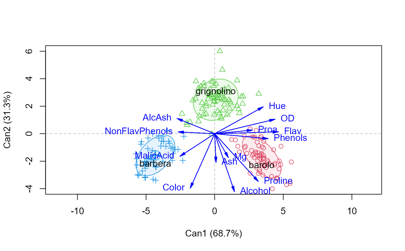
plot(Wine.can, ellipse=TRUE)
#> Vector scale factor set to 5.168

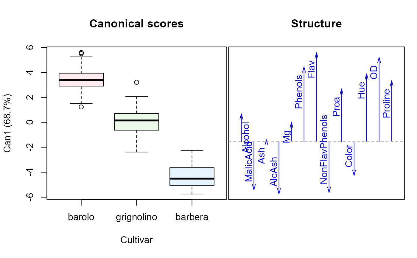
plot(Wine.can, which=1)