Canonical discriminant analysis

candisc performs a generalized canonical discriminant analysis for one term in a multivariate linear model (i.e., an mlm object), computing canonical scores and vectors. It represents a transformation of the original variables into a canonical space of maximal differences for the term, controlling for other model terms.

Usage

candisc(mod, ...)

# S3 method for class 'mlm'
candisc(mod, term, type = "2", manova, ndim = rank, ...)

# S3 method for class 'candisc'
print(x, digits = max(getOption("digits") - 2, 3), LRtests = TRUE, ...)

# S3 method for class 'candisc'
summary(
  object,
  means = TRUE,
  scores = FALSE,
  coef = c("std"),
  ndim,
  digits = max(getOption("digits") - 2, 4),
  ...
)

# S3 method for class 'candisc'
coef(object, type = c("std", "raw", "structure"), ...)

# S3 method for class 'candisc'
scores(x, ...)

# S3 method for class 'candisc'
plot(
  x,
  which = 1:2,
  conf = 0.95,
  col,
  pch,
  scale,
  asp = 1,
  var.col = "blue",
  var.lwd = par("lwd"),
  var.labels,
  var.cex = 1,
  var.pos,
  rev.axes = c(FALSE, FALSE),
  ellipse = FALSE,
  ellipse.prob = 0.68,
  fill.alpha = 0.1,
  prefix = "Can",
  suffix = TRUE,
  titles.1d = c("Canonical scores", "Structure"),
  points.1d = FALSE,
  ...
)

Arguments

mod: An mlm object, such as computed by lm() with a multivariate response
...: arguments to be passed down. In particular, type="n" can be used with the plot method to suppress the display of canonical scores.
term: the name of one term from mod for which the canonical analysis is performed.
type: type of test for the model term, one of: "II", "III", "2", or "3"
manova: the Anova.mlm object corresponding to mod. Normally, this is computed internally by Anova(mod)
ndim: Number of dimensions to store in (or retrieve from, for the summary method) the means, structure, scores and coeffs.* components. The default is the rank of the H matrix for the hypothesis term.
digits: significant digits to print.
LRtests: logical; should likelihood ratio tests for the canonical dimensions be printed?
object, x: A candisc object
means: Logical value used to determine if canonical means are printed
scores: Logical value used to determine if canonical scores are printed
coef: Type of coefficients printed by the summary method. Any one or more of "std", "raw", or "structure"
which: A vector of one or two integers, selecting the canonical dimension(s) to plot. If the canonical structure for a term has ndim==1, or length(which)==1, a 1D representation of canonical scores and structure coefficients is produced by the plot method. Otherwise, a 2D plot is produced.
conf: Confidence coefficient for the confidence circles around canonical means plotted in the plot method
col: A vector of the unique colors to be used for the levels of the term in the plot method, one for each level of the term. In this version, you should assign colors and point symbols explicitly, rather than relying on the somewhat arbitrary defaults, based on grDevices::palette().
pch: A vector of the unique point symbols to be used for the levels of the term in the plot method
scale: Scale factor for the variable vectors in canonical space. If not specified, a scale factor is calculated to make the variable vectors approximately fill the plot space.
asp: Aspect ratio for the plot method. The asp=1 (the default) assures that the units on the horizontal and vertical axes are the same, so that lengths and angles of the variable vectors are interpretable.
var.col: Color used to plot variable vectors
var.lwd: Line width used to plot variable vectors
var.labels: Optional vector of variable labels to replace variable names in the plots
var.cex: Character expansion size for variable labels in the plots
var.pos: Position(s) of variable vector labels wrt. the end point. If not specified, the labels are out-justified left and right with respect to the end points.
rev.axes: Logical, a vector of length(which). TRUE causes the orientation of the canonical scores and structure coefficients to be reversed along a given axis.
ellipse: Draw data ellipses for canonical scores?
ellipse.prob: Coverage probability for the data ellipses
fill.alpha: Transparency value for the color used to fill the ellipses. Use fill.alpha to draw the ellipses unfilled.
prefix: Prefix used to label the canonical dimensions plotted
suffix: Suffix for labels of canonical dimensions. If suffix=TRUE the percent of hypothesis (H) variance accounted for by each canonical dimension is added to the axis label.
titles.1d: A character vector of length 2, containing titles for the panels used to plot the canonical scores and structure vectors, for the case in which there is only one canonical dimension.
points.1d: Logical value for plot.candisc when only one canonical dimension.

Value

An object of class candisc with the following components:

dfh: hypothesis degrees of freedom for term
dfe: error degrees of freedom for the mlm
rank: number of non-zero eigenvalues of \(HE^{-1}\)
eigenvalues: eigenvalues of \(HE^{-1}\)
canrsq: squared canonical correlations
pct: A vector containing the percentages of the canrsq of their total.
ndim: Number of canonical dimensions stored in the means, structure and coeffs.* components
means: A data.frame containing the class means for the levels of the factor(s) in the term
factors: A data frame containing the levels of the factor(s) in the term
term: name of the term
terms: A character vector containing the names of the terms in the mlm object
coeffs.raw: A matrix containing the raw canonical coefficients
coeffs.std: A matrix containing the standardized canonical coefficients
structure: A matrix containing the canonical structure coefficients on ndim dimensions, i.e., the correlations between the original variates and the canonical scores. These are sometimes referred to as Total Structure Coefficients.
scores: A data frame containing the predictors in the mlm model and the canonical scores on ndim dimensions. These are calculated as Y \%*\% coeffs.raw, where Y contains the standardized response variables.

Details

In typical usage, the term should be a factor or interaction corresponding to a multivariate test with 2 or more degrees of freedom for the null hypothesis.

Canonical discriminant analysis is typically carried out in conjunction with a one-way MANOVA design. It represents a linear transformation of the response variables into a canonical space in which (a) each successive canonical variate produces maximal separation among the groups (e.g., maximum univariate F statistics), and (b) all canonical variates are mutually uncorrelated. For a one-way MANOVA with g groups and p responses, there are dfh = min( g-1, p) such canonical dimensions, and tests, initially stated by Bartlett (1938) allow one to determine the number of significant canonical dimensions.

Computational details for the one-way case are described in Cooley & Lohnes (1971), and in the SAS/STAT User's Guide, "The CANDISC procedure: Computational Details," http://support.sas.com/documentation/cdl/en/statug/63962/HTML/default/viewer.htm#statug_candisc_sect012.htm.

A generalized canonical discriminant analysis extends this idea to a general multivariate linear model. Analysis of each term in the mlm produces a rank \(df_h\) H matrix sum of squares and crossproducts matrix that is tested against the rank \(df_e\) E matrix by the standard multivariate tests (Wilks' Lambda, Hotelling-Lawley trace, Pillai trace, Roy's maximum root test). For any given term in the mlm, the generalized canonical discriminant analysis amounts to a standard discriminant analysis based on the H matrix for that term in relation to the full-model E matrix.

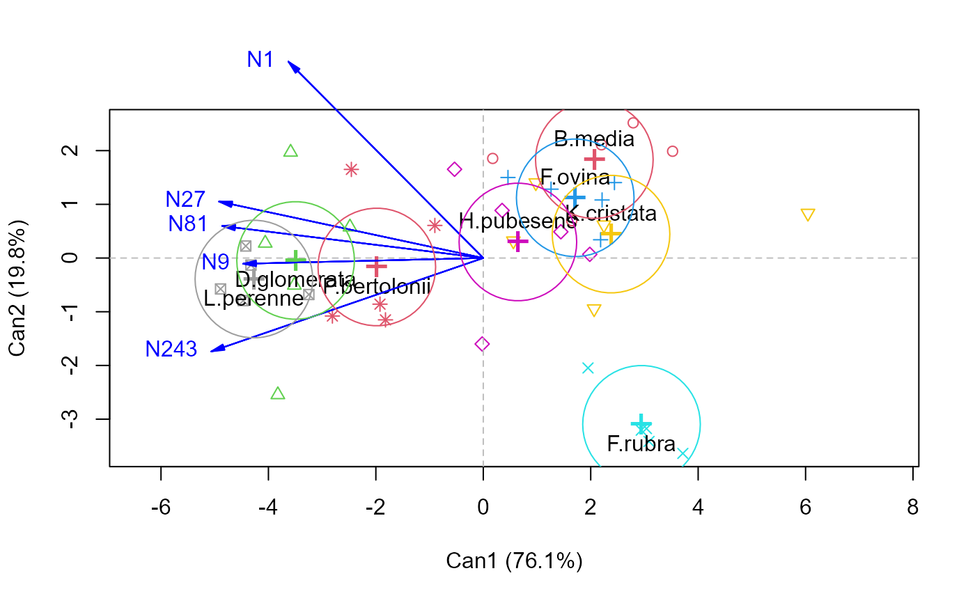
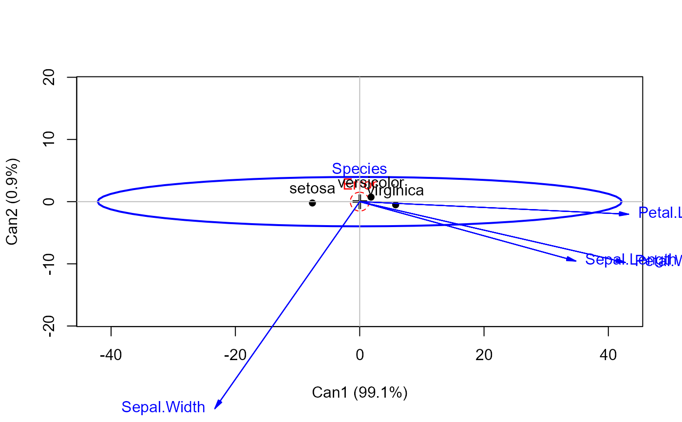
The plot method for candisc objects is typically a 2D plot, similar to a biplot. It shows the canonical scores for the groups defined by the term as points and the canonical structure coefficients as vectors from the origin.

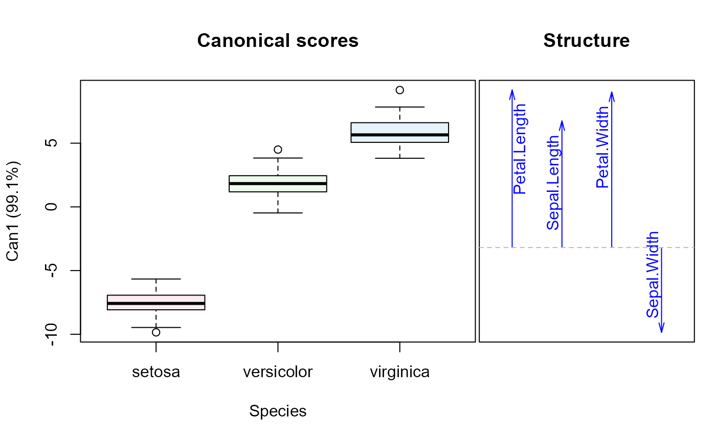
If the canonical structure for a term has ndim==1, or length(which)==1, the 1D representation consists of a boxplot of canonical scores and a vector diagram showing the magnitudes of the structure coefficients.

Methods (by class)

candisc(mlm): "mlm" method.

Methods (by generic)

print(candisc): print() method for "candisc" objects.
summary(candisc): summary() method for "candisc" objects.
coef(candisc): coef() method for "candisc" objects.
scores(candisc): scores() method for "candisc" objects.
plot(candisc): "plot" method.

References

Bartlett, M. S. (1938). Further aspects of the theory of multiple regression. Proc. Cambridge Philosophical Society 34, 33-34.

Cooley, W.W. & Lohnes, P.R. (1971). Multivariate Data Analysis, New York: Wiley.

Gittins, R. (1985). Canonical Analysis: A Review with Applications in Ecology, Berlin: Springer.

Author

Michael Friendly and John Fox

Examples


grass.mod <- lm(cbind(N1,N9,N27,N81,N243) ~ Block + Species, data=Grass)
car::Anova(grass.mod, test="Wilks")
#> 
#> Type II MANOVA Tests: Wilks test statistic
#>         Df test stat approx F num Df  den Df    Pr(>F)    
#> Block    4   0.33721   1.5620     20  80.549   0.08372 .  
#> Species  7   0.01570   4.9756     35 103.389 1.039e-10 ***
#> ---
#> Signif. codes:  0 '***' 0.001 '**' 0.01 '*' 0.05 '.' 0.1 ' ' 1

grass.can1 <-candisc(grass.mod, term="Species")
print(grass.can1)
#> 
#> Canonical Discriminant Analysis for Species:
#> 
#>     CanRsq Eigenvalue Difference   Percent Cumulative
#> 1 0.909573   10.05859     7.4384 76.094937     76.095
#> 2 0.723775    2.62024     7.4384 19.822550     95.917
#> 3 0.297819    0.42413     7.4384  3.208645     99.126
#> 4 0.093087    0.10264     7.4384  0.776506     99.903
#> 5 0.012706    0.01287     7.4384  0.097362    100.000
#> 
#> Test of H0: The canonical correlations in the 
#> current row and all that follow are zero
#> 
#>   LR test stat approx F numDF  denDF   Pr(> F)    
#> 1      0.01570   5.7853    35 120.22 2.162e-13 ***
#> 2      0.17367   2.7800    24 102.38 0.0001923 ***
#> 3      0.62873   1.0156    15  83.22 0.4478651    
#> 4      0.89539   0.4402     8  62.00 0.8922329    
#> 5      0.98729   0.1373     3  32.00 0.9370206    
#> ---
#> Signif. codes:  0 '***' 0.001 '**' 0.01 '*' 0.05 '.' 0.1 ' ' 1

plot(grass.can1, var.lwd = 2)
#> Vector scale factor set to 5.545


# library(heplots)
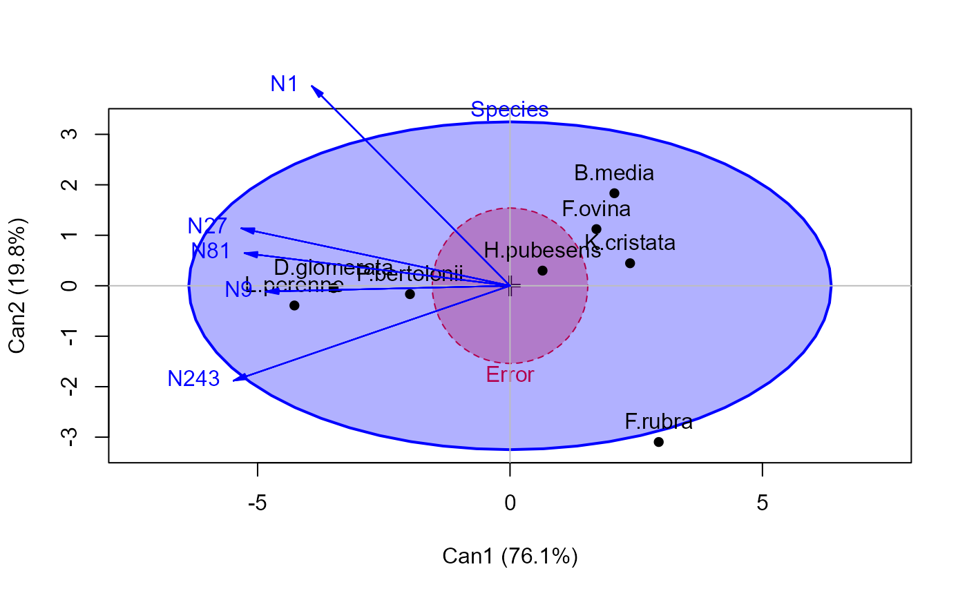
heplot(grass.can1, scale=6, fill=TRUE)


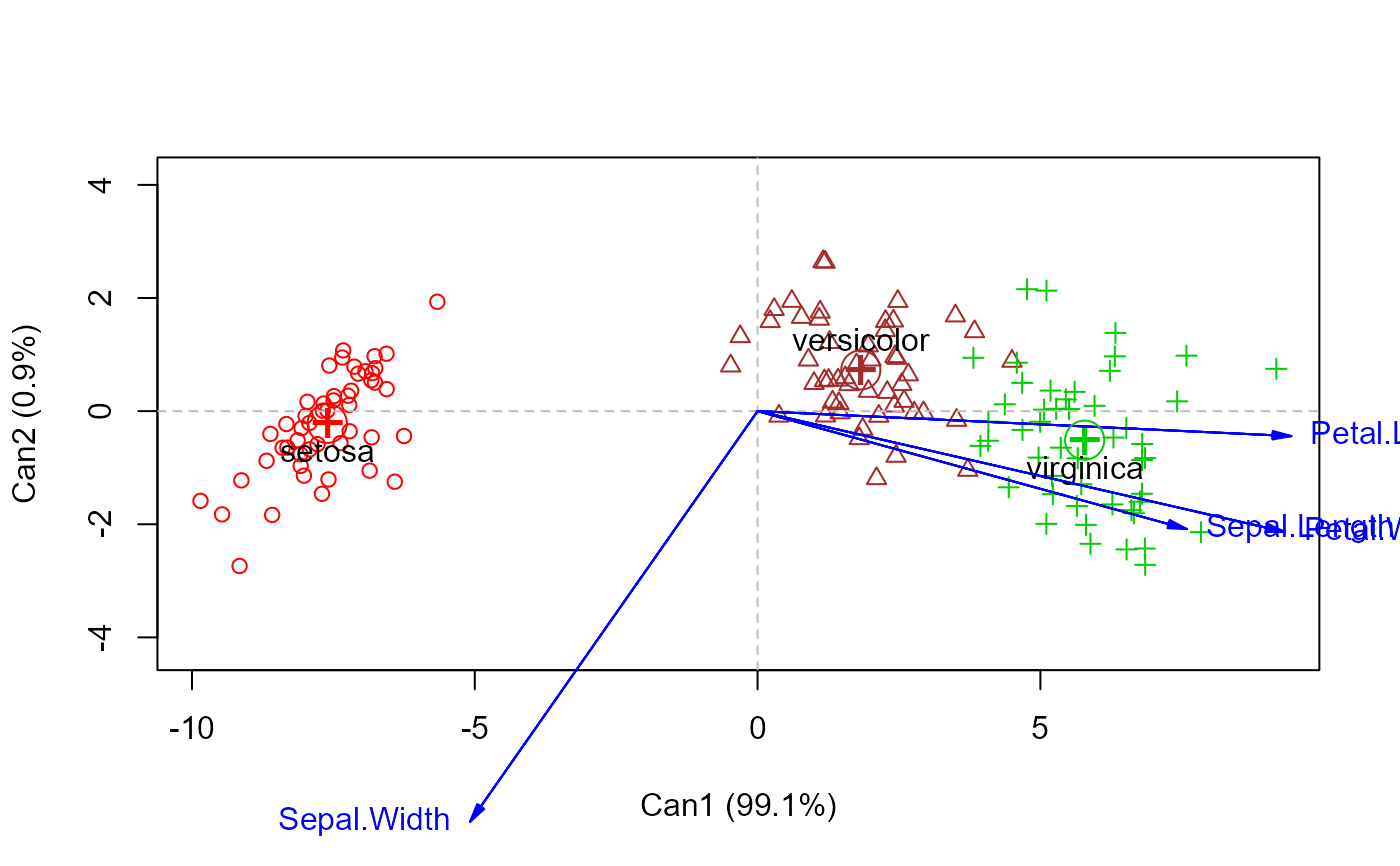
# iris data
iris.mod <- lm(cbind(Petal.Length, Sepal.Length, Petal.Width, Sepal.Width) ~ Species, data=iris)
iris.can <- candisc(iris.mod, data=iris)
#-- assign colors and symbols corresponding to species
col <- c("red", "brown", "green3")
pch <- 1:3
plot(iris.can, col=col, pch=pch)
#> Vector scale factor set to 9.58


heplot(iris.can)

#> Vector scale factor set to  43.914 

# 1-dim plot
iris.can1 <- candisc(iris.mod, data=iris, ndim=1)
plot(iris.can1)