Two-Dimensional HE Plots

This function plots ellipses representing the hypothesis and error sums-of-squares-and-products matrices for terms and linear hypotheses in a multivariate linear model. These include MANOVA models (all explanatory variables are factors), multivariate regression (all quantitative predictors), MANCOVA models, homogeneity of regression, as well as repeated measures designs treated from a multivariate perspective.

Usage

heplot(mod, ...)

# S3 method for mlm
heplot(
  mod,
  terms,
  hypotheses,
  term.labels = TRUE,
  hyp.labels = TRUE,
  err.label = "Error",
  label.pos = NULL,
  variables = 1:2,
  error.ellipse = !add,
  factor.means = !add,
  grand.mean = !add,
  remove.intercept = TRUE,
  type = c("II", "III", "2", "3"),
  idata = NULL,
  idesign = NULL,
  icontrasts = c("contr.sum", "contr.poly"),
  imatrix = NULL,
  iterm = NULL,
  markH0 = !is.null(iterm),
  manova,
  size = c("evidence", "effect.size"),
  level = 0.68,
  alpha = 0.05,
  segments = 60,
  center.pch = "+",
  center.cex = 2,
  col = getOption("heplot.colors", c("red", "blue", "black", "darkgreen", "darkcyan",
    "magenta", "brown", "darkgray")),
  lty = 2:1,
  lwd = 1:2,
  fill = FALSE,
  fill.alpha = 0.3,
  xlab,
  ylab,
  main = "",
  xlim,
  ylim,
  axes = TRUE,
  offset.axes,
  add = FALSE,
  verbose = FALSE,
  warn.rank = FALSE,
  ...
)

Arguments

mod: a model object of class "mlm".
...: arguments to pass down to plot, text, and points.
terms: a logical value or character vector of terms in the model for which to plot hypothesis matrices; if missing or TRUE, defaults to all terms; if FALSE, no terms are plotted.
hypotheses: optional list of linear hypotheses for which to plot hypothesis matrices; hypotheses are specified as for the linearHypothesis function in the car package; the list elements can be named, in which case the names are used.
term.labels: logical value or character vector of names for the terms to be plotted. If TRUE (the default) the names of the terms are used; if FALSE, term labels are not plotted.
hyp.labels: logical value or character vector of names for the hypotheses to be plotted. If TRUE (the default) the names of components of the list of hypotheses are used; if FALSE, hypothesis labels are not plotted.
err.label: Label for the error ellipse
label.pos: Label position, a vector of integers (in 0:4) or character strings (in c("center", "bottom", "left", "top", "right"), or in c("C", "S", "W", "N", "E") use in labeling ellipses, recycled as necessary. Values of 1, 2, 3 and 4, respectively indicate positions below, to the left of, above and to the right of the max/min coordinates of the ellipse; the value 0 specifies the centroid of the ellipse object. The default, label.pos=NULL uses the correlation of the ellipse to determine "top" (r>=0) or "bottom" (r<0). Even more flexible options are described in label.ellipse
variables: indices or names of the two response variables to be plotted; defaults to 1:2.
error.ellipse: if TRUE, plot the error ellipse; defaults to TRUE, if the argument add is FALSE (see below).
factor.means: logical value or character vector of names of factors for which the means are to be plotted, or TRUE or FALSE; defaults to TRUE, if the argument add is FALSE (see below).
grand.mean: if TRUE, plot the centroid for all of the data; defaults to TRUE, if the argument add is FALSE (see below).
remove.intercept: if TRUE (the default), do not plot the ellipse for the intercept even if it is in the MANOVA table.
type: ``type'' of sum-of-squares-and-products matrices to compute; one of "II", "III", "2", or "3", where "II" is the default (and "2" is a synonym).
idata: an optional data frame giving a factor or factors defining the intra-subject model for multivariate repeated-measures data. See Friendly (2010) and Details of Anova for an explanation of the intra-subject design and for further explanation of the other arguments relating to intra-subject factors.
idesign: a one-sided model formula using the ``data'' in idata and specifying the intra-subject design for repeated measure models.
icontrasts: names of contrast-generating functions to be applied by default to factors and ordered factors, respectively, in the within-subject ``data''; the contrasts must produce an intra-subject model matrix in which different terms are orthogonal. The default is c("contr.sum", "contr.poly").
imatrix: In lieu of idata and idesign, you can specify the intra-subject design matrix directly via imatrix, in the form of list of named elements. Each element gives the columns of the within-subject model matrix for an intra-subject term to be tested, and must have as many rows as there are responses; the columns of the within-subject model matrix for different terms must be mutually orthogonal.
iterm: For repeated measures designs, you must specify one intra-subject term (a character string) to select the SSPE (E) matrix used in the HE plot. Hypothesis terms plotted include the iterm effect as well as all interactions of iterm with terms.
markH0: A logical value (or else a list of arguments to mark.H0) used to draw cross-hairs and a point indicating the value of a point null hypothesis. The default is TRUE if iterm is non-NULL.
manova: optional Anova.mlm object for the model; if absent a MANOVA is computed. Specifying the argument can therefore save computation in repeated calls.
size: how to scale the hypothesis ellipse relative to the error ellipse; if "evidence", the default, the scaling is done so that a ``significant'' hypothesis ellipse at level alpha extends outside of the error ellipse; if "effect.size", the hypothesis ellipse is on the same scale as the error ellipse.
level: equivalent coverage of ellipse for normally-distributed errors, defaults to 0.68, giving a standard 1 SD bivariate ellipse.
alpha: significance level for Roy's greatest-root test statistic; if size="evidence", then the hypothesis ellipse is scaled so that it just touches the error ellipse at the specified alpha level; a larger hypothesis ellipse somewhere in the space of the response variables therefore indicates statistical significance; defaults to 0.05.
segments: number of line segments composing each ellipse; defaults to 60.
center.pch: character to use in plotting the centroid of the data; defaults to "+".
center.cex: size of character to use in plotting the centroid of the data; defaults to 2.
col: a color or vector of colors to use in plotting ellipses; the first color is used for the error ellipse; the remaining colors --- recycled as necessary --- are used for the hypothesis ellipses. A single color can be given, in which case it is used for all ellipses. For convenience, the default colors for all heplots produced in a given session can be changed by assigning a color vector via options(heplot.colors =c(...). Otherwise, the default colors are c("red", "blue", "black", "darkgreen", "darkcyan", "magenta", "brown", "darkgray").
lty: vector of line types to use for plotting the ellipses; the first is used for the error ellipse, the rest --- possibly recycled --- for the hypothesis ellipses; a single line type can be given. Defaults to 2:1.
lwd: vector of line widths to use for plotting the ellipses; the first is used for the error ellipse, the rest --- possibly recycled --- for the hypothesis ellipses; a single line width can be given. Defaults to 1:2.
fill: A logical vector indicating whether each ellipse should be filled or not. The first value is used for the error ellipse, the rest --- possibly recycled --- for the hypothesis ellipses; a single fill value can be given. Defaults to FALSE for backward compatibility. See Details below.
fill.alpha: Alpha transparency for filled ellipses, a numeric scalar or vector of values within [0,1], where 0 means fully transparent and 1 means fully opaque.
xlab: x-axis label; defaults to name of the x variable.
ylab: y-axis label; defaults to name of the y variable.
main: main plot label; defaults to "".
xlim: x-axis limits; if absent, will be computed from the data.
ylim: y-axis limits; if absent, will be computed from the data.
axes: Whether to draw the x, y axes; defaults to TRUE
offset.axes: proportion to extend the axes in each direction if computed from the data; optional.
add: if TRUE, add to the current plot; the default is FALSE. If TRUE, the error ellipse is not plotted.
verbose: if TRUE, print the MANOVA table and details of hypothesis tests; the default is FALSE.
warn.rank: if TRUE, do not suppress warnings about the rank of the hypothesis matrix when the ellipse collapses to a line; the default is FALSE.

Value

The function invisibly returns an object of class "heplot", with coordinates for the various hypothesis ellipses and the error ellipse, and the limits of the horizontal and vertical axes. These may be useful for adding additional annotations to the plot, using standard plotting functions. (No methods for manipulating these objects are currently available.)

The components are:

H: a list containing the coordinates of each ellipse for the hypothesis terms
E: a matrix containing the coordinates for the error ellipse
center: x,y coordinates of the centroid
xlim: x-axis limits
ylim: y-axis limits
radius: the radius for the unit circles used to generate the ellipses

Details

The heplot function plots a representation of the covariance ellipses for hypothesized model terms and linear hypotheses (H) and the corresponding error (E) matrices for two response variables in a multivariate linear model (mlm).

The plot helps to visualize the nature and dimensionality response variation on the two variables jointly in relation to error variation that is summarized in the various multivariate test statistics (Wilks' Lambda, Pillai trace, Hotelling-Lawley trace, Roy maximum root). Roy's maximum root test has a particularly simple visual interpretation, exploited in the size="evidence" version of the plot. See the description of argument alpha.

For a 1 df hypothesis term (a quantitative regressor, a single contrast or parameter test), the H matrix has rank 1 (one non-zero latent root of \(H E^{-1}\)) and the H "ellipse" collapses to a degenerate line.

Typically, you fit a mlm with mymlm <- lm(cbind(y1, y2, y3, ...) ~ modelterms), and plot some or all of the modelterms with heplot(mymlm, ...). Arbitrary linear hypotheses related to the terms in the model (e.g., contrasts of an effect) can be included in the plot using the hypotheses argument. See linearHypothesis for details.

For repeated measure designs, where the response variables correspond to one or more variates observed under a within-subject design, between-subject effects and within-subject effects must be plotted separately, because the error terms (E matrices) differ. When you specify an intra-subject term (iterm), the analysis and HE plots amount to analysis of the matrix Y of responses post-multiplied by a matrix M determined by the intra-subject design for that term. See Friendly (2010) or the vignette("repeated") in this package for an extended discussion and examples.

The related candisc package provides functions for visualizing a multivariate linear model in a low-dimensional view via a generalized canonical discriminant analyses. heplot.candisc and heplot3d.candisc provide a low-rank 2D (or 3D) view of the effects for a given term in the space of maximum discrimination.

When an element of fill is TRUE, the ellipse outline is drawn using the corresponding color in col, and the interior is filled with a transparent version of this color specified in fill.alpha. To produce filled (non-degenerate) ellipses without the bounding outline, use a value of lty=0 in the corresponding position.

References

Friendly, M. (2006). Data Ellipses, HE Plots and Reduced-Rank Displays for Multivariate Linear Models: SAS Software and Examples Journal of Statistical Software, 17(6), 1--42. https://www.jstatsoft.org/v17/i06/, DOI: 10.18637/jss.v017.i06

Friendly, M. (2007). HE plots for Multivariate General Linear Models. Journal of Computational and Graphical Statistics, 16(2) 421--444. http://datavis.ca/papers/jcgs-heplots.pdf

Friendly, Michael (2010). HE Plots for Repeated Measures Designs. Journal of Statistical Software, 37(4), 1-40. DOI: 10.18637/jss.v037.i04.

Fox, J., Friendly, M. & Weisberg, S. (2013). Hypothesis Tests for Multivariate Linear Models Using the car Package. The R Journal, 5(1), https://journal.r-project.org/archive/2013-1/fox-friendly-weisberg.pdf.

Friendly, M. & Sigal, M. (2014) Recent Advances in Visualizing Multivariate Linear Models. Revista Colombiana de Estadistica, 37, 261-283.

Examples


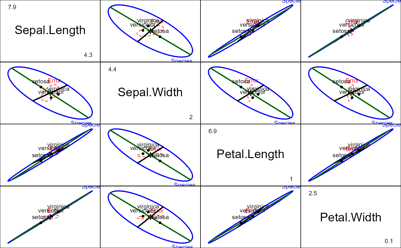
## iris data
contrasts(iris$Species) <- matrix(c(0,-1,1, 2, -1, -1), 3,2)
contrasts(iris$Species)
#>            [,1] [,2]
#> setosa        0    2
#> versicolor   -1   -1
#> virginica     1   -1

iris.mod <- lm(cbind(Sepal.Length, Sepal.Width, Petal.Length, Petal.Width) ~
Species, data=iris)

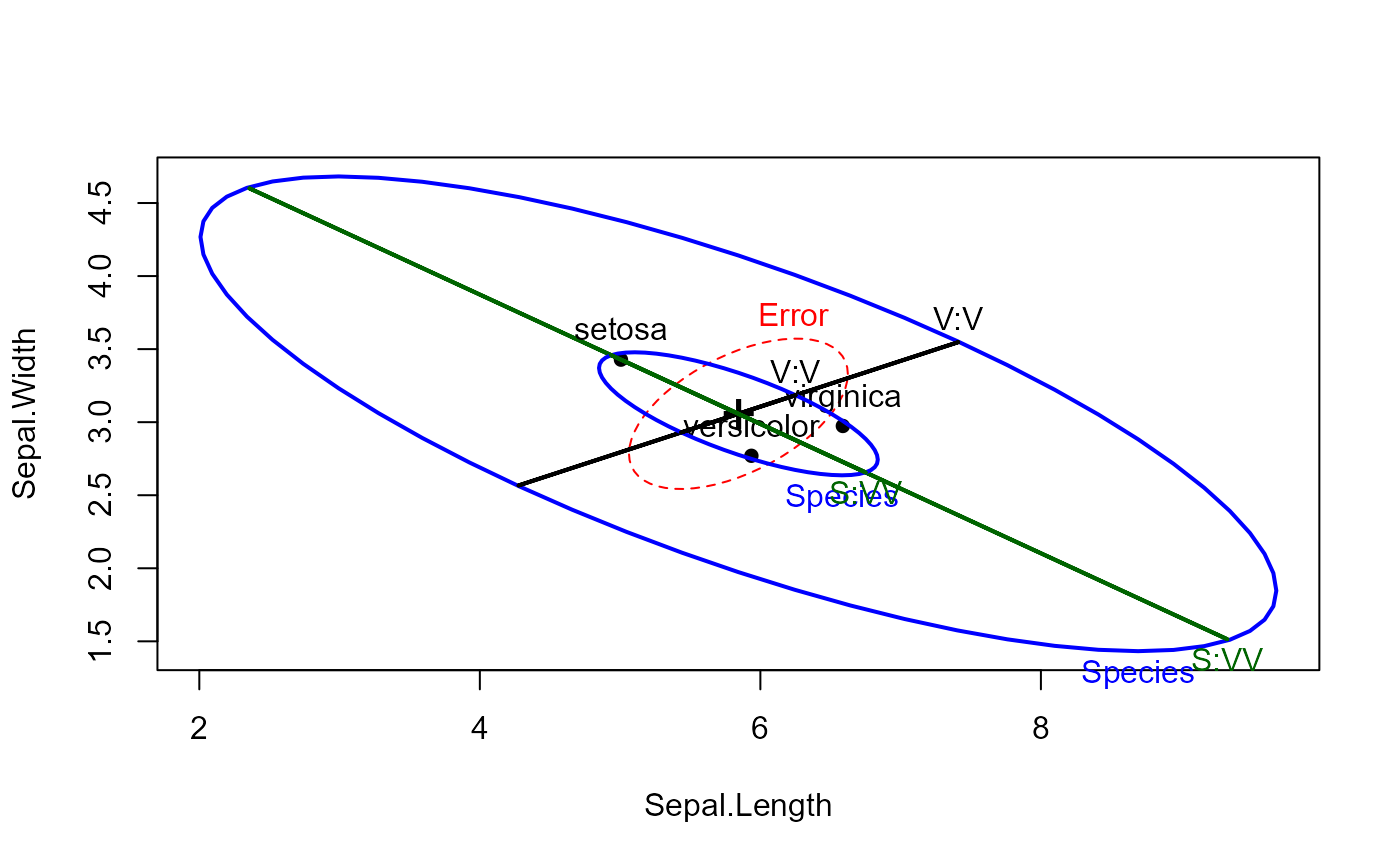
hyp <- list("V:V"="Species1","S:VV"="Species2")
heplot(iris.mod, hypotheses=hyp)
# compare with effect-size scaling
heplot(iris.mod, hypotheses=hyp, size="effect", add=TRUE)


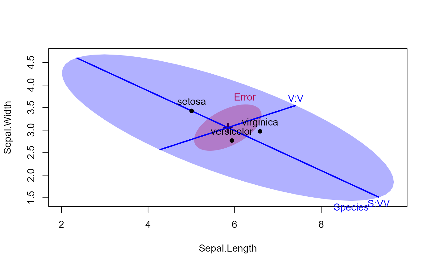
# try filled ellipses; include contrasts
heplot(iris.mod, hypotheses=hyp, fill=TRUE, 
       fill.alpha=0.2, col=c("red", "blue"))

heplot(iris.mod, hypotheses=hyp, fill=TRUE, 
       col=c("red", "blue"), lty=c(0,0,1,1))


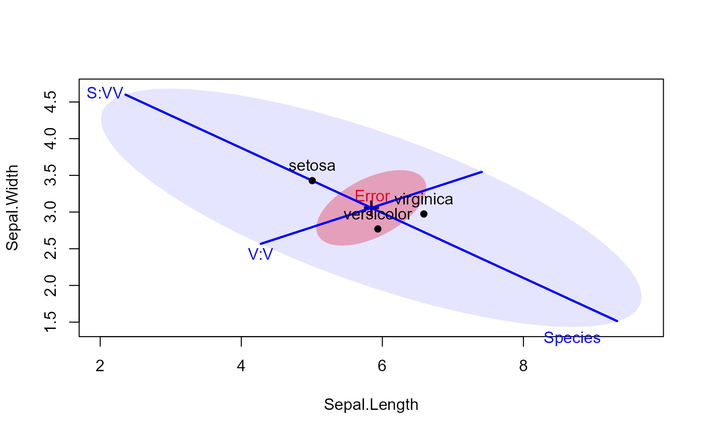
# vary label position and fill.alpha
heplot(iris.mod, hypotheses=hyp, fill=TRUE, fill.alpha=c(0.3,0.1), col=c("red", "blue"), 
       lty=c(0,0,1,1), label.pos=0:3)


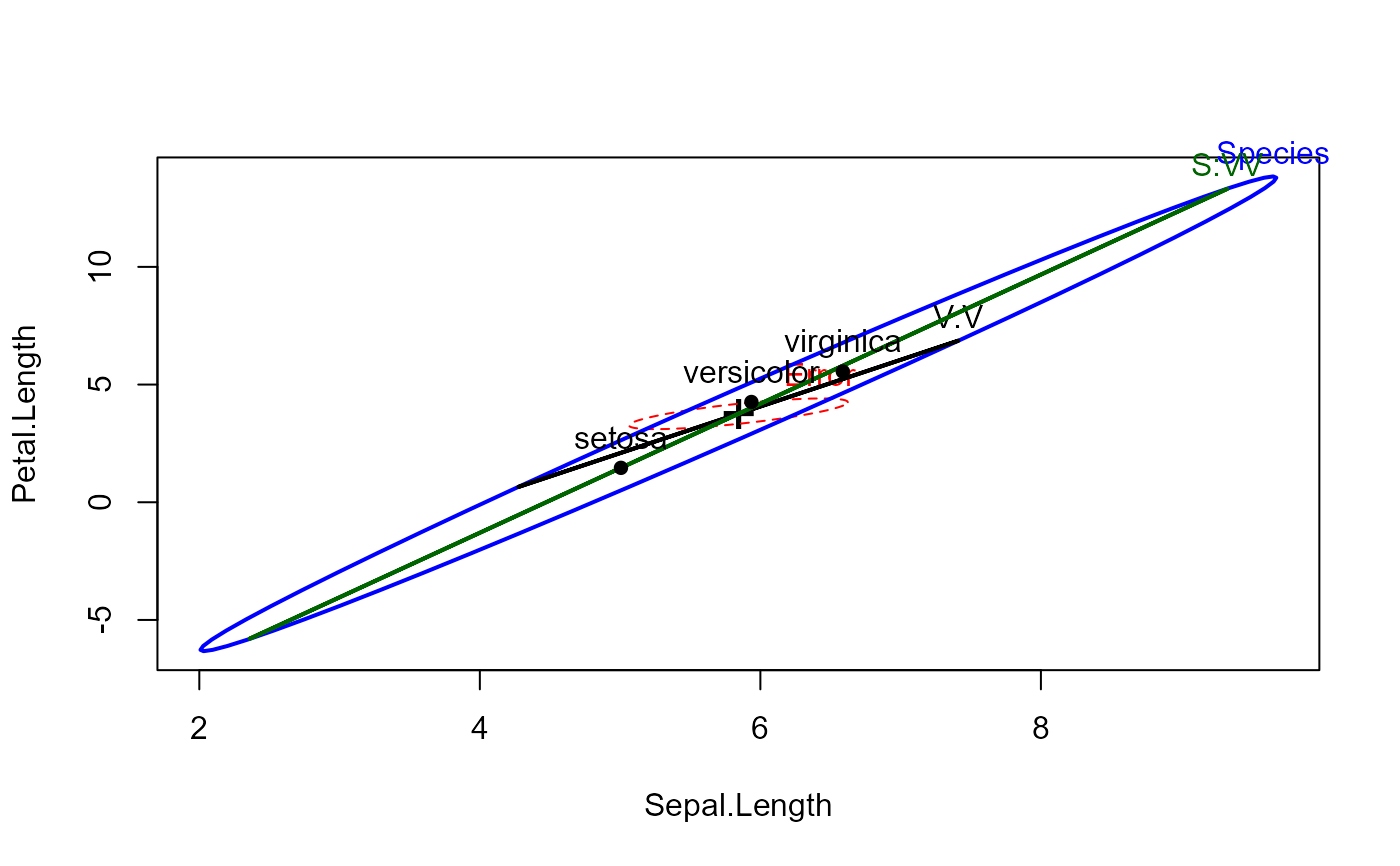
# what is returned?
hep <-heplot(iris.mod, variables=c(1,3),  hypotheses=hyp)

str(hep)
#> List of 6
#>  $ H     :List of 3
#>   ..$ Species: num [1:61, 1:2] 9.66 9.68 9.66 9.6 9.5 ...
#>   .. ..- attr(*, "dimnames")=List of 2
#>   .. .. ..$ : NULL
#>   .. .. ..$ : chr [1:2] "Sepal.Length" "Petal.Length"
#>   ..$ V:V    : num [1:61, 1:2] 7.41 7.4 7.38 7.33 7.27 ...
#>   .. ..- attr(*, "dimnames")=List of 2
#>   .. .. ..$ : NULL
#>   .. .. ..$ : chr [1:2] "Sepal.Length" "Petal.Length"
#>   ..$ S:VV   : num [1:61, 1:2] 9.33 9.31 9.25 9.16 9.03 ...
#>   .. ..- attr(*, "dimnames")=List of 2
#>   .. .. ..$ : NULL
#>   .. .. ..$ : chr [1:2] "Sepal.Length" "Petal.Length"
#>  $ E     : num [1:61, 1:2] 6.62 6.62 6.61 6.59 6.56 ...
#>   ..- attr(*, "dimnames")=List of 2
#>   .. ..$ : NULL
#>   .. ..$ : chr [1:2] "Sepal.Length" "Petal.Length"
#>  $ center: Named num [1:2] 5.84 3.76
#>   ..- attr(*, "names")= chr [1:2] "Sepal.Length" "Petal.Length"
#>  $ xlim  : Named num [1:2] 2.01 9.68
#>   ..- attr(*, "names")= chr [1:2] "Sepal.Length" "Sepal.Length"
#>  $ ylim  : Named num [1:2] -6.33 13.84
#>   ..- attr(*, "names")= chr [1:2] "Petal.Length" "Petal.Length"
#>  $ radius: num 1.52
#>  - attr(*, "class")= chr "heplot"

# all pairs
pairs(iris.mod, hypotheses=hyp, hyp.labels=FALSE)



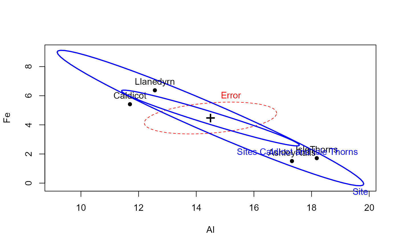
## Pottery data, from car package
data(Pottery, package = "carData")
pottery.mod <- lm(cbind(Al, Fe, Mg, Ca, Na) ~ Site, data=Pottery)
heplot(pottery.mod)
heplot(pottery.mod, terms=FALSE, add=TRUE, col="blue", 
  hypotheses=list(c("SiteCaldicot = 0", "SiteIsleThorns=0")),
  hyp.labels="Sites Caldicot and Isle Thorns")


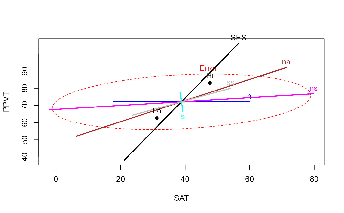
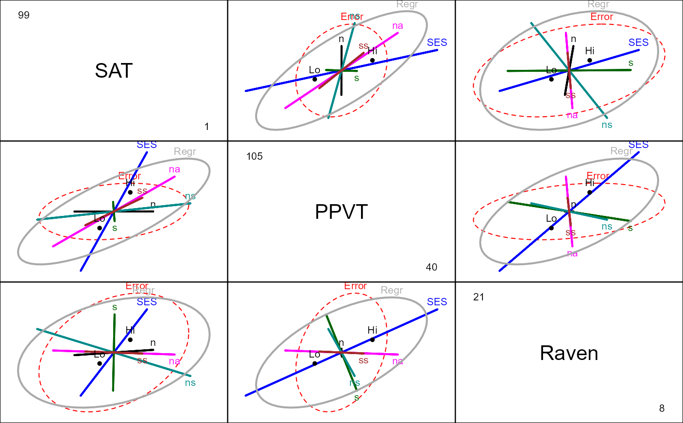
## Rohwer data, multivariate multiple regression/ANCOVA
#-- ANCOVA, assuming equal slopes
rohwer.mod <- lm(cbind(SAT, PPVT, Raven) ~ SES + n + s + ns + na + ss, data=Rohwer)
car::Anova(rohwer.mod)
#> 
#> Type II MANOVA Tests: Pillai test statistic
#>     Df test stat approx F num Df den Df    Pr(>F)    
#> SES  1   0.37853  12.1818      3     60 2.507e-06 ***
#> n    1   0.04030   0.8400      3     60  0.477330    
#> s    1   0.09271   2.0437      3     60  0.117307    
#> ns   1   0.19283   4.7779      3     60  0.004729 ** 
#> na   1   0.23134   6.0194      3     60  0.001181 ** 
#> ss   1   0.04990   1.0504      3     60  0.376988    
#> ---
#> Signif. codes:  0 '***' 0.001 '**' 0.01 '*' 0.05 '.' 0.1 ' ' 1
col <- c("red", "black", "blue", "cyan", "magenta", "brown", "gray")
heplot(rohwer.mod, col=col)


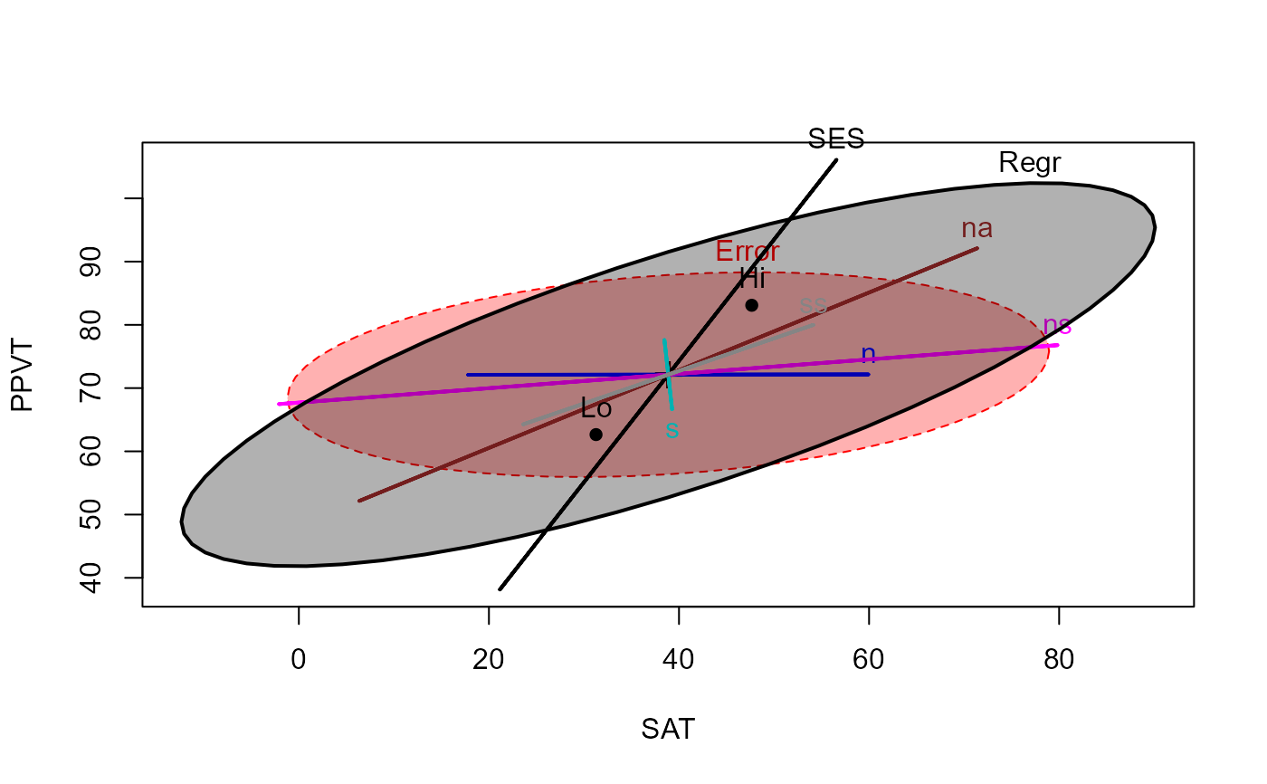
# Add ellipse to test all 5 regressors
heplot(rohwer.mod, hypotheses=list("Regr" = c("n", "s", "ns", "na", "ss")), 
       col=col, fill=TRUE)

# View all pairs
pairs(rohwer.mod, hypotheses=list("Regr" = c("n", "s", "ns", "na", "ss")))

# or 3D plot

if(requireNamespace("rgl")){
col <- c("pink", "black", "blue", "cyan", "magenta", "brown", "gray")
heplot3d(rohwer.mod, hypotheses=list("Regr" = c("n", "s", "ns", "na", "ss")), col=col)
}