U. S. Crimes — crime • ggbiplot

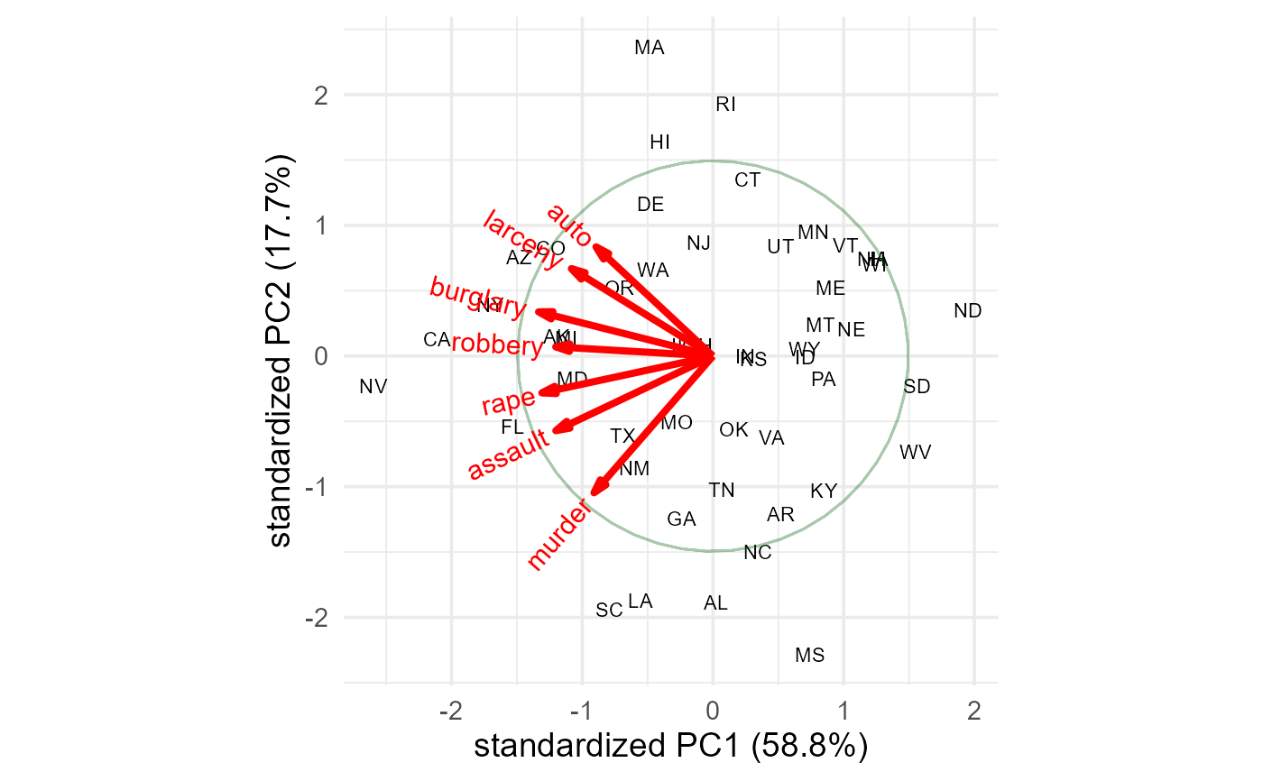
This dataset gives rates of occurrence (per 100,000 people) various serious crimes in each of the 50 U. S. states, originally from the United States Statistical Abstracts (1970). The data were analyzed by John Hartigan (1975) in his book Clustering Algorithms and were later reanalyzed by Friendly (1991).

Usage

data(crime)

Format

A data frame with 50 observations on the following 10 variables.

state: state name, a character vector
murder: a numeric vector
rape: a numeric vector
robbery: a numeric vector
assault: a numeric vector
burglary: a numeric vector
larceny: a numeric vector
auto: auto thefts, a numeric vector
st: state abbreviation, a character vector
region: region of the U.S., a factor with levels Northeast South North Central West

Source

The data are originally from the United States Statistical Abstracts (1970). This dataset also appears in the SAS/Stat Sample library, Getting Started Example for PROC PRINCOMP, https://support.sas.com/documentation/onlinedoc/stat/ex_code/131/princgs.html, from which the current copy was derived.

References

Friendly, M. (1991). SAS System for Statistical Graphics. SAS Institute.

Hartigan, J. A. (1975). Clustering Algorithms. John Wiley and Sons.

Examples

data(crime)
library(ggplot2)
crime.pca <- 
  crime |> 
  dplyr::select(where(is.numeric)) |>
  prcomp(scale. = TRUE)

ggbiplot(crime.pca,
     labels = crime$st ,
     circle = TRUE,
     varname.size = 4,
     varname.color = "red") +
 theme_minimal(base_size = 14)