Univariate versus Multivariate Influence

Influence measures are well-known for linear models with a single response variable. These measures, such as Cook’s D, DFFITS and DFBETAS assess the impact of each observation by calculating measures of the change in regression coefficients, fitted values, etc. when that observation is omitted from the data (Belsley, Kuh and Welsch (1980), Cook and Weisberg (1982)).

For models with two or more response variables, the functions in the mvinfluence package calculate natural extensions of the standard measures hatvalues, cooks.distance according to the theory presented in Barrett & Ling (1992). However, multivariate influence turns out to be more interesting and complex than just the collection of diagnostics for the separate responses, as this example illustrates.

Load packages

library(tibble)      # Simple Data Frames
library(ggplot2)     # Create Elegant Data Visualisations Using the Grammar of Graphics
library(car)         # Companion to Applied Regression
library(mvinfluence) # Influence Measures and Diagnostic Plots for Multivariate Linear Models
library(patchwork)   # The Composer of Plots
library(rgl)         # 3D Visualization Using OpenGL
rgl::setupKnitr(autoprint = TRUE)    # render rgl plots in a knitr document

A Toy Example

This example, from Barrett (2003), considers the simplest case, of one predictor (x) and two response variables, y1 and y2.

Toy <- tibble(
   case = 1:9,
   x =  c(1,    1,    2,    2,    3,    3,    4,    4,    10),
   y1 = c(0.10, 1.90, 1.00, 2.95, 2.10, 4.00, 2.95, 4.95, 10.00),
   y2 = c(0.10, 1.80, 1.00, 2.93, 2.00, 4.10, 3.05, 4.93, 10.00)
)

A quick peek at the data indicates that y1 and y2 are nearly perfectly correlated. Both of these are linear with x and there is one extreme point (case 9). Looking at these pairwise plots doesn’t suggest that anything is terribly wrong.

car::scatterplotMatrix(~y1 + y2 + x, data=Toy, cex=2,
        col = "blue", pch = 16,
        id = list(n=1, cex=2), 
        regLine = list(lwd = 2, col="red"),
        smooth = FALSE)

We can view the data in 3D, using car::scatter3d(). The regression plane shown is that for the model y1 ~ y2 + x. The plot is interactive: you can rotate and zoom using the mouse to see the views shown in the scatterplots. If you rotate the plot so the regression plane becomes a line, you can see that the data ellipsoid is essentially flat.

car::scatter3d(y1 ~ y2 + x, data=Toy,
               ellipsoid = TRUE,              # show the data ellipsoid
               radius = c(rep(1,8), 2),       # make case 9 larger
               grid.col = "pink", grid.lines = 10, 
               fill = FALSE,
               id = list(n=1), offset=2
               )
rgl::rglwidget()

Models

We fit the univariate models with y1 and y2 separately and then the multivariate model.

Toy.lm1 <- lm(y1 ~ x, data=Toy)
Toy.lm2 <- lm(y2 ~ x, data=Toy)
Toy.mlm <- lm(cbind(y1, y2) ~ x, data=Toy)

Note that the coefficients in the multivariate model Toy.mlm are identical to those in the separate univariate models for y1 and y2. That is, \(\mathbf{B} = [ \mathbf{b_{y1}} , \mathbf{b_{y2}} ]\), as if the univariate models were fit individually.

coef(Toy.lm1)
#> (Intercept)           x 
#>   -0.003704    0.999444

coef(Toy.lm2)
#> (Intercept)           x 
#>    -0.02556     1.00467

coef(Toy.mlm)
#>                    y1       y2
#> (Intercept) -0.003704 -0.02556
#> x            0.999444  1.00467

However, the test for predictors differ, because the multivariate tests take the correlation between y1 and y2 into account.

car::Anova(Toy.lm1)
#> Anova Table (Type II tests)
#> 
#> Response: y1
#>           Sum Sq Df F value  Pr(>F)    
#> x           59.9  1    57.2 0.00013 ***
#> Residuals    7.3  7                    
#> ---
#> Signif. codes:  0 '***' 0.001 '**' 0.01 '*' 0.05 '.' 0.1 ' ' 1

car::Anova(Toy.lm2)
#> Anova Table (Type II tests)
#> 
#> Response: y2
#>           Sum Sq Df F value  Pr(>F)    
#> x           60.6  1    58.1 0.00012 ***
#> Residuals    7.3  7                    
#> ---
#> Signif. codes:  0 '***' 0.001 '**' 0.01 '*' 0.05 '.' 0.1 ' ' 1

car::Anova(Toy.mlm)
#> 
#> Type II MANOVA Tests: Pillai test statistic
#>   Df test stat approx F num Df den Df Pr(>F)   
#> x  1     0.893     25.1      2      6 0.0012 **
#> ---
#> Signif. codes:  0 '***' 0.001 '**' 0.01 '*' 0.05 '.' 0.1 ' ' 1

Cook’s D

First, let’s examine the Cook’s D statistics for the models. Note that the function cooks.distance() invokes stats::cooks.distance.lm() for the univariate response models, but invokes mvinfluence::cooks.distance.mlm() for the multivariate model.

The only thing remarkable here is for case 9: The univariate Cook’s Ds, D1 and D2 are very small, yet the multivariate statistic, D12 is over 10 times the next smallest value.

df <- Toy
df$D1  <- cooks.distance(Toy.lm1)
df$D2  <- cooks.distance(Toy.lm2)
df$D12 <- cooks.distance(Toy.mlm)

df
#> # A tibble: 9 x 7
#>    case     x    y1    y2      D1      D2    D12
#>   <int> <dbl> <dbl> <dbl>   <dbl>   <dbl>  <dbl>
#> 1     1     1  0.1   0.1  0.121   0.118   0.125 
#> 2     2     1  1.9   1.8  0.124   0.103   0.298 
#> 3     3     2  1     1    0.0901  0.0886  0.0906
#> 4     4     2  2.95  2.93 0.0829  0.0819  0.0831
#> 5     5     3  2.1   2    0.0548  0.0673  0.182 
#> 6     6     3  4     4.1  0.0692  0.0852  0.232 
#> 7     7     4  2.95  3.05 0.0793  0.0651  0.203 
#> 8     8     4  4.95  4.93 0.0665  0.0643  0.0690
#> 9     9    10 10    10    0.00159 0.00830 3.22

We can see how case 9 stands out in the influence plots. It has an extreme hat value, but, because it’s residual is very small, it does not have much influence on the fitted models for either y1 or y2. Neither of these plots suggest that anything is terribly wrong with the univariate models.

ip1 <- car::influencePlot(Toy.lm1, id = list(cex=1.5), cex.lab = 1.5)
ip2 <- car::influencePlot(Toy.lm2, id = list(cex=1.5), cex.lab = 1.5)

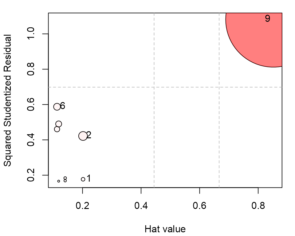
Contrast these results with what we get for the model for y1 and y2 jointly. In the multivariate version, influencePlot.mlm plots the squared studentized residual (denoted Q in the output) against the hat value. Case 9 stands out as wildly influential.

influencePlot(Toy.mlm, id.n=2)

#>        H      Q  CookD      L      R
#> 1 0.2019 0.1769 0.1250 0.2529 0.2216
#> 2 0.2019 0.4219 0.2981 0.2529 0.5286
#> 6 0.1130 0.5873 0.2322 0.1273 0.6621
#> 9 0.8519 1.0816 3.2249 5.7500 7.3010

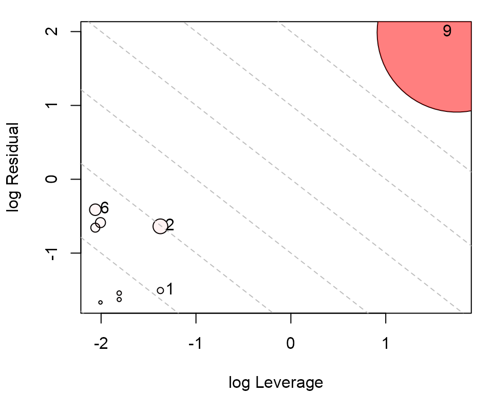
An alternative form of the multivariate influence plot uses the leverage (L) and residual (R) components. Because influence is the product of leverage and residual, a plot of \(\log(L)\) versus \(\log(R)\) has the attractive property that contours of constant Cook’s distance fall on diagonal lines with slope = -1. Adjacent reference lines represent constant multiples of influence.

influencePlot(Toy.mlm, id.n=2, type = 'LR')

DFBETAS

The DFBETAS statistics give the estimated change in the regression coefficients when each case is deleted in turn. We can gain some insight as to why case 9 is unremarkable in the univariate regressions by plotting these. The values come from stats::dfbetas and return the standardized values.

db1 <- as.data.frame(dfbetas(Toy.lm1))
gg1 <- ggplot(data = db1, aes(x=`(Intercept)`, y=x, label=rownames(db1))) +
  geom_point(size=1.5) +
  geom_label(size=6, fill="pink") +
  xlab(expression(paste("Deletion Intercept  ", b[0]))) +
  ylab(expression(paste("Deletion Slope  ", b[1]))) +
  ggtitle("dfbetas for y1") +
  theme_bw(base_size = 16)

db2 <- as.data.frame(dfbetas(Toy.lm2))
gg2 <- ggplot(data = db2, aes(x=`(Intercept)`, y=x, label=rownames(db2))) +
  geom_point(size=1.5) +
  geom_label(size=6, fill="pink") +
  xlab(expression(paste("Deletion Intercept  ", b[0]))) +
  ylab(expression(paste("Deletion Slope  ", b[1]))) +
  ggtitle("dfbetas for y2") +
  theme_bw(base_size = 16)

gg1 + gg2

The values for case 9 are nearly (0, 0) in both plots, indicating that deleting this case has negligible effect in both univariate regressions.

What happended here?

This example was contrived to show a situation where no cases were influential in the univariate models, but case 9 appeared very influential in the multivariate model. Why did this happen?

My colleague, John Fox, pointed out that the problem arose from the very high correlation between y1 and y2:

with(Toy, cor(y1, y2))
#> [1] 0.9997

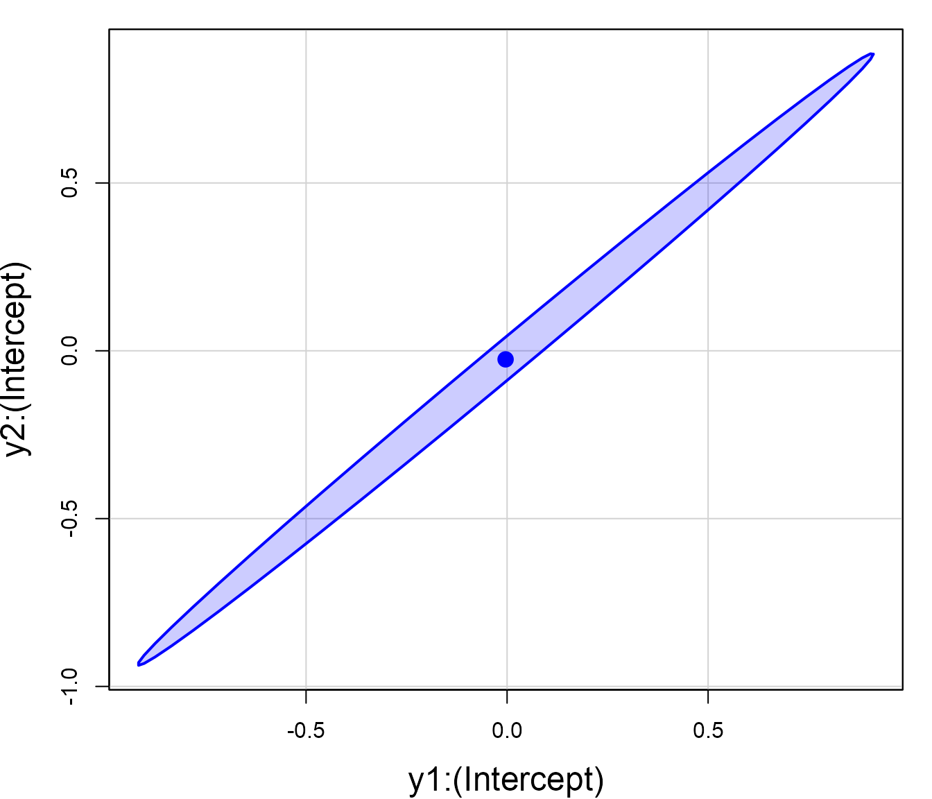
As a consequence, the covariance matrix of the multivariate regression coefficient vector is very ill-conditioned as can be seen by converting the covariance matrix to correlations:

(corr <- cov2cor(vcov(Toy.mlm)))
#>                y1:(Intercept)    y1:x y2:(Intercept)    y2:x
#> y1:(Intercept)         1.0000 -0.7906         0.9973 -0.7885
#> y1:x                  -0.7906  1.0000        -0.7885  0.9973
#> y2:(Intercept)         0.9973 -0.7885         1.0000 -0.7906
#> y2:x                  -0.7885  0.9973        -0.7906  1.0000

This appear in the correlations between the two intercept terms {y1,y2}:(Intercept) and the two slope terms, {y1,y2}:x, and can be visualized by confidence ellipses for pairs of these parameters:

par(mar = c(4, 4, 1, 1)+.1)
car::confidenceEllipse(Toy.mlm, which=c(1,3), levels = 0.68,
                       xlab = row.names(corr)[1], 
                       ylab=row.names(corr)[3],
                       fill = TRUE, fill.alpha = 0.2,
                       cex.lab = 1.5)

car::confidenceEllipse(Toy.mlm, which=c(2,4), levels = 0.68,
                       xlab = row.names(corr)[2], 
                       ylab=row.names(corr)[4],
                       fill = TRUE, fill.alpha = 0.2,
                       cex.lab = 1.5)

Although each of the y1 and y2 values for the high-leverage cases are in-line with the univariate regressions (and thus have small univariate Cook’s Ds), the ill-conditioning magnifies small discrepancies in their positions, making the multivariate Cook’s D larger.

References

Barrett, B. E. and Ling, R. F. (1992). General Classes of Influence Measures for Multivariate Regression. Journal of the American Statistical Association, 87(417), 184-191.

Barrett, B. E. (2003). Understanding Influence in Multivariate Regression. Communications in Statistics – Theory and Methods, 32, 3, 667-680.

Belsley, D. A., Kuh, E. and Welsch, R. E. (1980). Regression Diagnostics. New York: Wiley.

Cook, R. D. and Weisberg, S. (1982). Residuals and Influence in Regression. London: Chapman and Hall.

Lawrence, A. J. (1995). Deletion Influence and Masking in Regression. Journal of the Royal Statistical Society. Series B (Methodological) , 57, No. 1, pp. 181-189.

Michael Friendly