Companion to Arizona: monthly mean temperatures for three cities spanning a wide
range of latitudes along the East Coast (Laredo, TX; Washington, DC; Caribou, ME),
used by Tukey (1977) as a second example of a two-way (row + column) fit.
Format
a matrix of 7 rows (Month, Jan–July) and 3 columns (City: Laredo, Washington,
Caribou) where the value is mean monthly temperature in degrees F. The matrix has
a responseName attribute, "Temperature"
References
Tukey, J. W. (1977). Exploratory Data Analysis, Reading MA: Addison-Wesley. Exhibit 9 of chapter 10, p. 354
Examples
data(EastCoast)
# Using median polish
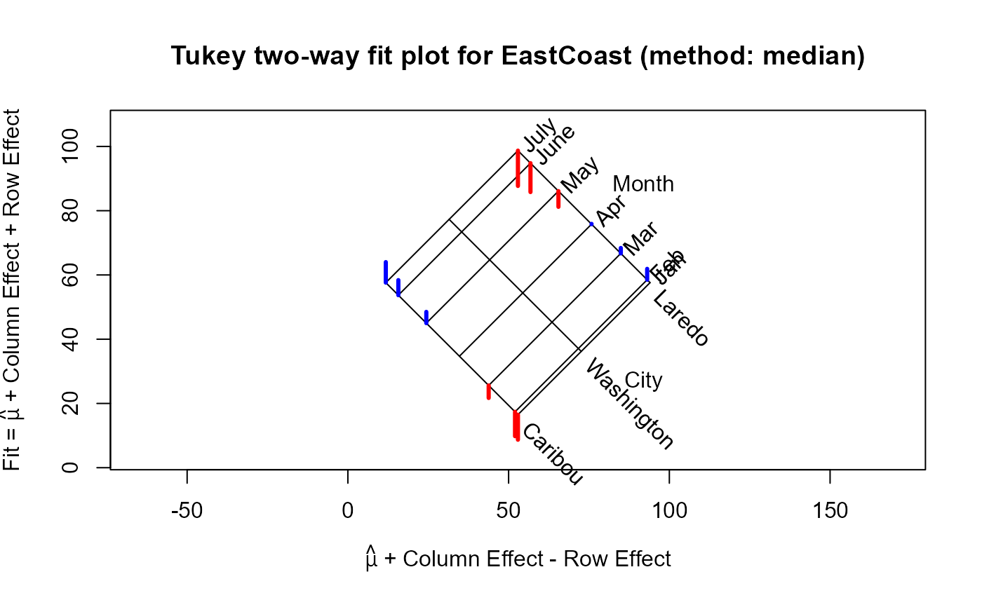
(EC.2way.med <- twoway(EastCoast, method="median"))
#>
#> Median polish decomposition (Dataset: "EastCoast"; Response: Temperature)
#> Residuals bordered by row effects, column effects, and overall
#>
#> City
#> Month Laredo Washington Caribou roweff
#> + ----- ----- ----- + -----
#> Jan | 0.0 0.0 -7.8 : -18.2
#> Feb | 3.4 0.0 -7.6 : -17.3
#> Mar | 1.7 0.0 -3.9 : -9.1
#> Apr | 0.1 0.0 0.0 : 0.0
#> May | -4.9 0.0 3.5 : 10.3
#> June | -9.0 0.0 4.7 : 19.0
#> July | -11.0 0.0 6.4 : 22.9
#> + ..... ..... ..... + .....
#> coleff | 21.4 0.0 -19.7 : 54.4
#>
plot(EC.2way.med)
 plot(EC.2way.med, which="diagnose")
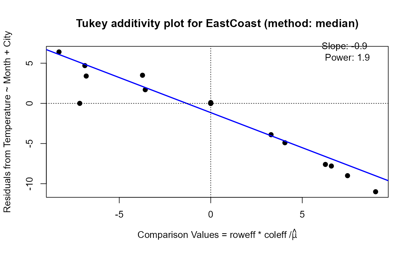 #> Slope of Residual on comparison value: -0.9
#> Suggested power transformation: 1.9
#> Ladder of powers transformation: square
# Using mean polish
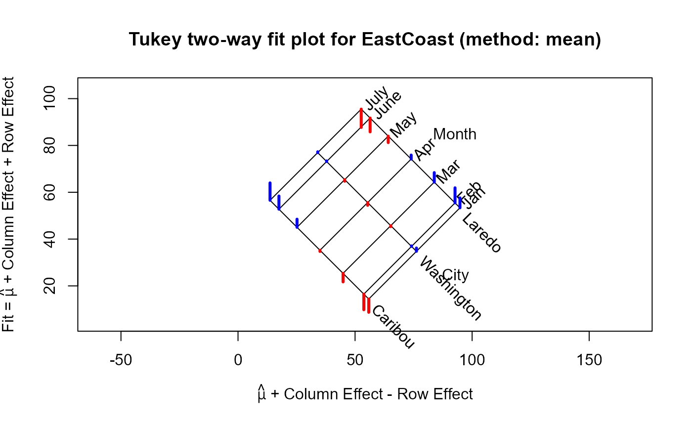
EC.2way.mean <- twoway(EastCoast)
plot(EC.2way.mean)
#> Slope of Residual on comparison value: -0.9
#> Suggested power transformation: 1.9
#> Ladder of powers transformation: square
# Using mean polish
EC.2way.mean <- twoway(EastCoast)
plot(EC.2way.mean)
 # Show the two ANOVAs
anova(EC.2way.mean)
#> Dataset: EastCoast; method: "mean"
#>
#> Analysis of Variance Table, assuming additivity
#>
#> Df Sum Sq Mean Sq F value Pr(>F)
#> Month 6 5222.4 870.40 27.655 2.339e-06 ***
#> City 2 5315.5 2657.76 84.443 8.524e-08 ***
#> Residuals 12 377.7 31.47
#> ---
#> Signif. codes: 0 '***' 0.001 '**' 0.01 '*' 0.05 '.' 0.1 ' ' 1
#>
#>
#> Analysis of Variance Table, allowing non-additivity
#>
#> Df Sum Sq Mean Sq F value Pr(>F)
#> Month 6 5222.4 870.40 548.70 5.728e-13 ***
#> City 2 5315.5 2657.76 1675.45 2.145e-14 ***
#> nonadd 1 360.2 360.24 227.09 1.085e-08 ***
#> pure error 11 17.4 1.59
#> ---
#> Signif. codes: 0 '***' 0.001 '**' 0.01 '*' 0.05 '.' 0.1 ' ' 1
# Show the two ANOVAs
anova(EC.2way.mean)
#> Dataset: EastCoast; method: "mean"
#>
#> Analysis of Variance Table, assuming additivity
#>
#> Df Sum Sq Mean Sq F value Pr(>F)
#> Month 6 5222.4 870.40 27.655 2.339e-06 ***
#> City 2 5315.5 2657.76 84.443 8.524e-08 ***
#> Residuals 12 377.7 31.47
#> ---
#> Signif. codes: 0 '***' 0.001 '**' 0.01 '*' 0.05 '.' 0.1 ' ' 1
#>
#>
#> Analysis of Variance Table, allowing non-additivity
#>
#> Df Sum Sq Mean Sq F value Pr(>F)
#> Month 6 5222.4 870.40 548.70 5.728e-13 ***
#> City 2 5315.5 2657.76 1675.45 2.145e-14 ***
#> nonadd 1 360.2 360.24 227.09 1.085e-08 ***
#> pure error 11 17.4 1.59
#> ---
#> Signif. codes: 0 '***' 0.001 '**' 0.01 '*' 0.05 '.' 0.1 ' ' 1