Counts of an insect for the combinations of 4 treatments and 6 areas of a field

Counts of numbers of an insect, Leptinotarsa decemlineata (the Colorado potato beetle), each of which is the sum for two plots treated alike, for all combinations of 4 treatments and 6 areas of the field chosen to be relatively homogeneous.

Format

a 4 x 6 matrix, where the rows are treatments and the columns are areas of a field.

Details

These data are used in Tukey (1977) Exhibit 1 of Ch 11 and throughout the chapter as examples of median polish. Because the data are counts, either a sqrt or log transformation would be reasonable.

References

Tukey, J. W. (1977). Exploratory Data Analysis, Reading MA: Addison-Wesley. Exhibit 1 of chapter 111

Examples

insect.2way <- twoway(insectCounts, method="median")
print(insect.2way, digits=2)
#> 
#> Median polish decomposition (Dataset: "insectCounts"; Response: Value)
#> Residuals bordered by row effects, column effects, and overall
#> 
#>         area
#> treat      area1   area2   area3   area4   area5   area6     roweff 
#>          + ------- ------- ------- ------- ------- ------- + -------
#>   t1     |   71.07   -2.54    0.39  394.50  -75.54   -1.50 :  252.00
#>   t2     |    2.86  -32.75   71.18   30.29 -135.75   -0.71 :  -60.79
#>   t3     | -171.71   45.68   -0.39  -30.29  106.68    0.71 :   60.79
#>   t4     |   -2.86    2.54   -7.54  -72.43   75.54   93.57 : -162.07
#>          + ....... ....... ....... ....... ....... ....... + .......
#>   coleff |  -26.84  -35.23   26.84   52.73   28.77 -116.27 :  195.77
#> 

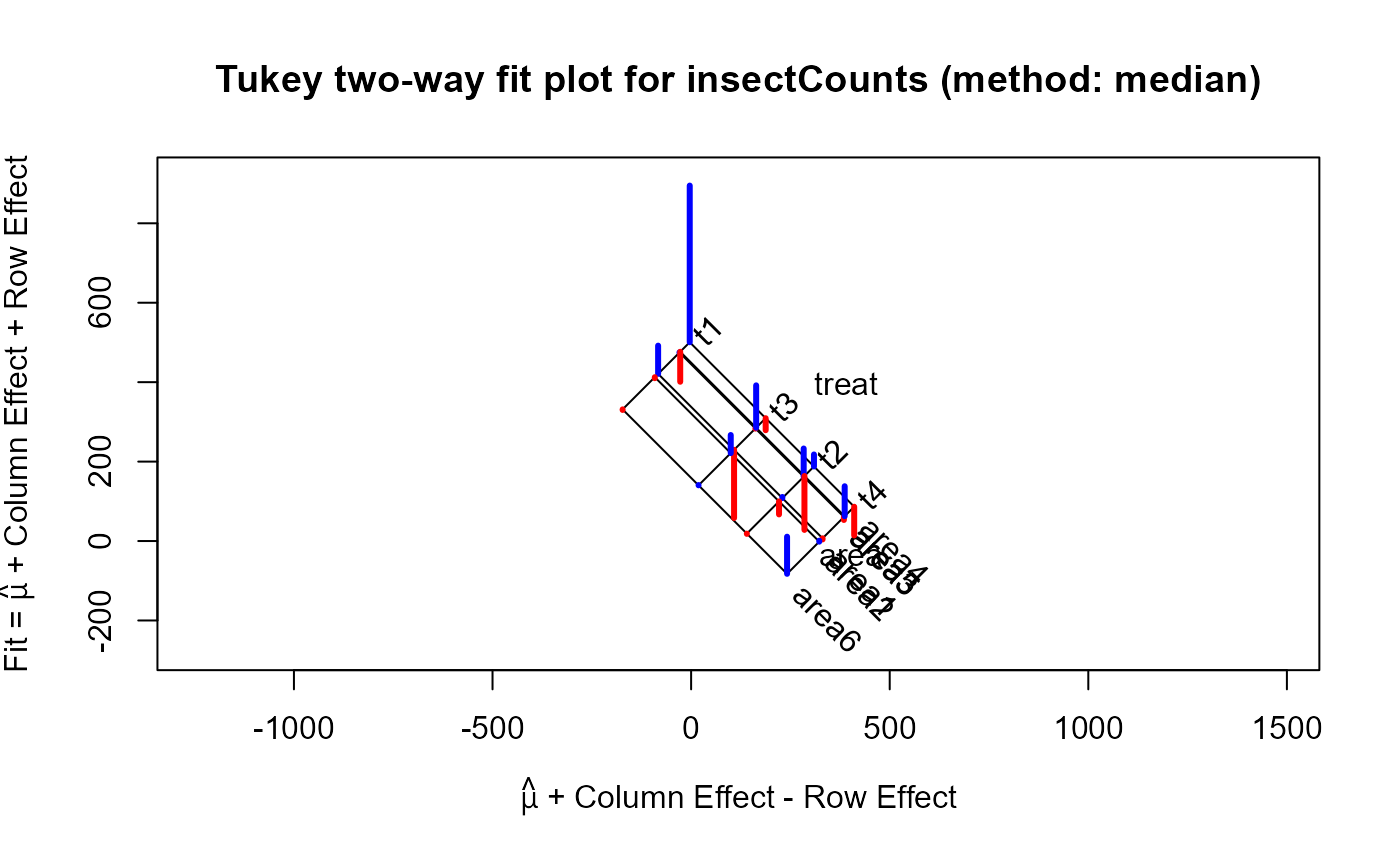
plot(insect.2way)

plot(insect.2way, which="diagnose")

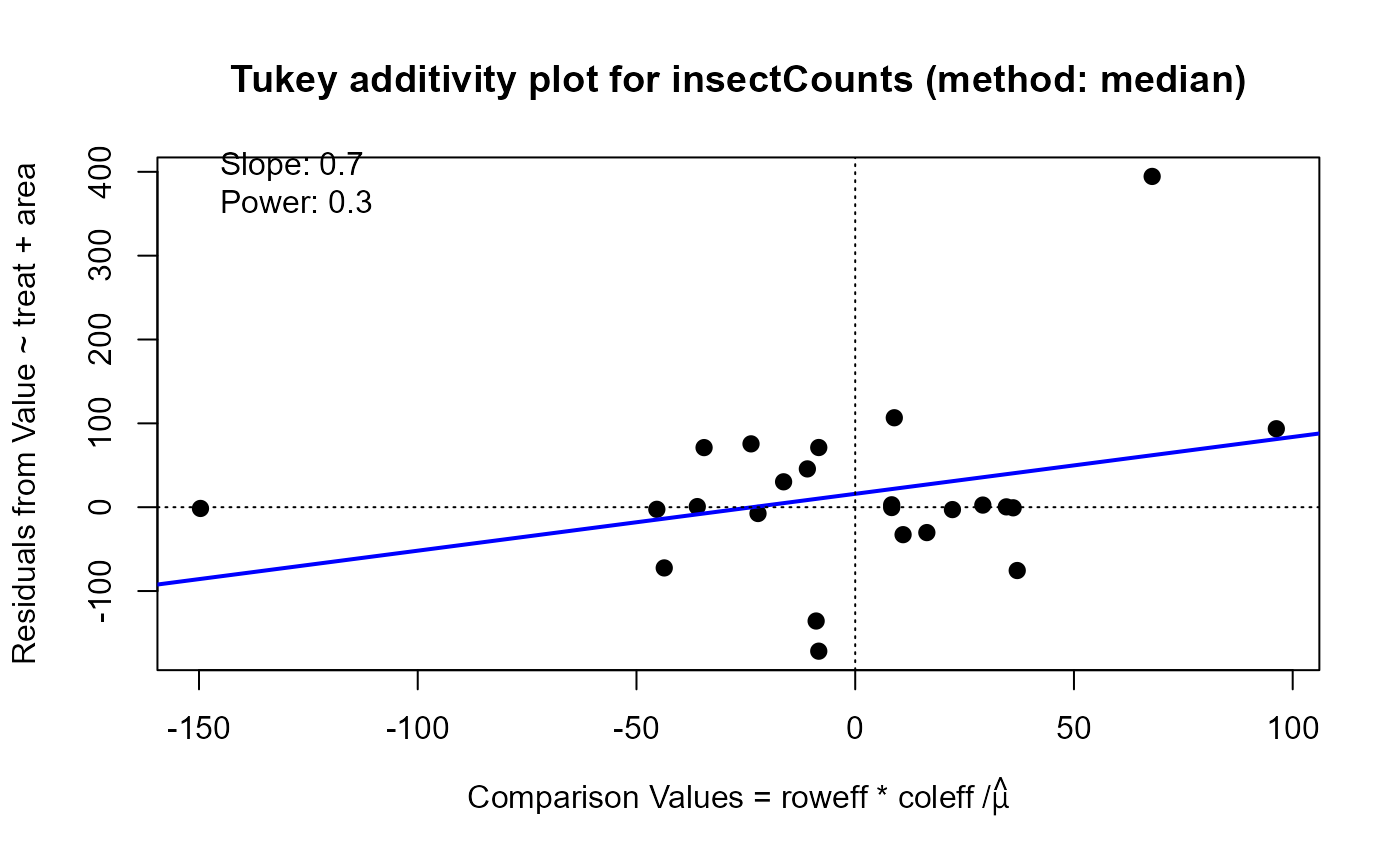#> Slope of Residual on comparison value:  0.7 
#> Suggested power transformation:         0.3 
#> Ladder of powers transformation:        cube root 

# try sqrt transformation
insect.sqrt <- twoway(sqrt(insectCounts), method="median")
print(insect.sqrt, digits=2)
#> 
#> Median polish decomposition (Dataset: "sqrt(insectCounts)"; Response: Value)
#> Residuals bordered by row effects, column effects, and overall
#> 
#>         area
#> treat      area1 area2 area3 area4 area5 area6   roweff
#>          + ----- ----- ----- ----- ----- ----- + ----- 
#>   t1     |  1.25  0.41 -2.78  5.07 -3.38 -0.34 :  9.12 
#>   t2     |  0.86 -0.41  1.94  1.17 -6.86 -3.02 : -2.14 
#>   t3     | -6.34  3.48 -0.78 -1.17  3.38  0.34 :  2.14 
#>   t4     | -0.86 -0.77  0.78 -3.03  6.42  2.88 : -8.96 
#>          + ..... ..... ..... ..... ..... ..... + ..... 
#>   coleff | -1.24 -2.33  2.41  2.68  1.23 -3.66 : 13.06 
#> 

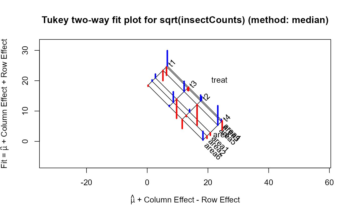
plot(insect.sqrt)

plot(insect.sqrt, which="diagnose")

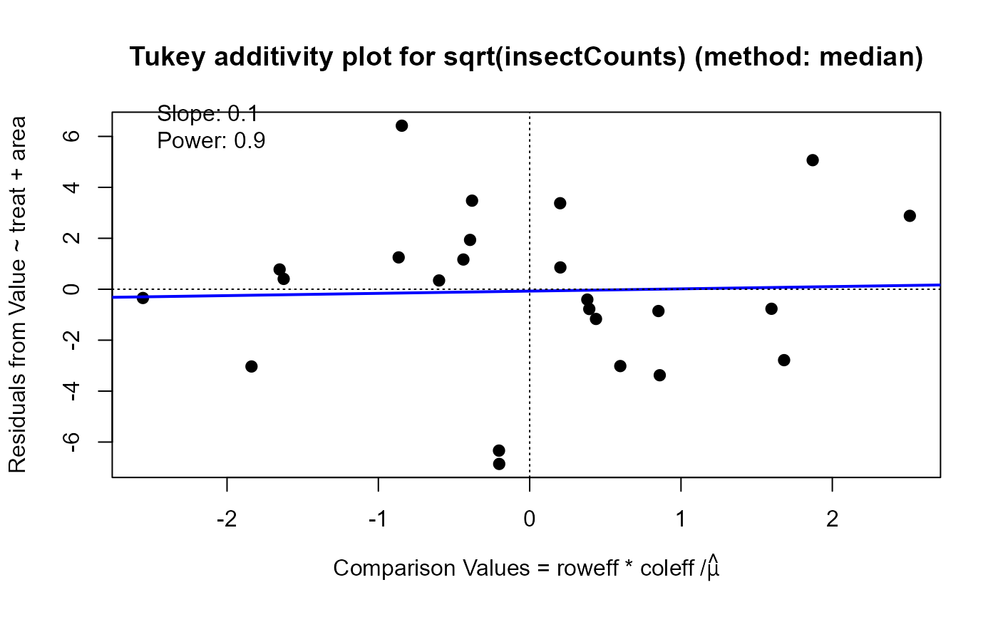#> Slope of Residual on comparison value:  0.1 
#> Suggested power transformation:         0.9 
#> Ladder of powers transformation:        no transformation