gaussianElimination demonstrates the algorithm of row reduction used for solving
systems of linear equations of the form \(A x = B\). Optional arguments verbose
and fractions may be used to see how the algorithm works.
Arguments
- A
coefficient matrix
- B
right-hand side vector or matrix. If
Bis a matrix, the result gives solutions for each column as the right-hand side of the equations with coefficients inA.- tol
tolerance for checking for 0 pivot
- verbose
logical; if
TRUE, print intermediate steps- latex
logical; if
TRUE, and verbose isTRUE, print intermediate steps using LaTeX equation outputs rather than R output- fractions
logical; if
TRUE, try to express non-integers as rational numbers, using thefractionsfunction; if you require greater accuracy, you can set thecycles(default 10) and/ormax.denominator(default 2000) arguments tofractionsas a global option, e.g.,options(fractions=list(cycles=100, max.denominator=10^4)).- x
matrix to print
- ...
arguments to pass down
Value
If B is absent, returns the reduced row-echelon form of A.
If B is present, returns the reduced row-echelon form of A, with the
same operations applied to B.
Examples
A <- matrix(c(2, 1, -1,
-3, -1, 2,
-2, 1, 2), 3, 3, byrow=TRUE)
b <- c(8, -11, -3)
gaussianElimination(A, b)
#> [,1] [,2] [,3] [,4]
#> [1,] 1 0 0 2
#> [2,] 0 1 0 3
#> [3,] 0 0 1 -1
gaussianElimination(A, b, verbose=TRUE, fractions=TRUE)
#>
#> Initial matrix:
#> Warning: Function is deprecated. See latexMatrix() and Eqn() for more recent approaches
#> [,1] [,2] [,3] [,4]
#> [1,] 2 1 -1 8
#> [2,] -3 -1 2 -11
#> [3,] -2 1 2 -3
#>
#> row: 1
#>
#> exchange rows 1 and 2
#> Warning: Function is deprecated. See latexMatrix() and Eqn() for more recent approaches
#> [,1] [,2] [,3] [,4]
#> [1,] -3 -1 2 -11
#> [2,] 2 1 -1 8
#> [3,] -2 1 2 -3
#>
#> multiply row 1 by -1/3
#> Warning: Function is deprecated. See latexMatrix() and Eqn() for more recent approaches
#> [,1] [,2] [,3] [,4]
#> [1,] 1 1/3 -2/3 11/3
#> [2,] 2 1 -1 8
#> [3,] -2 1 2 -3
#>
#> multiply row 1 by 2 and subtract from row 2
#> Warning: Function is deprecated. See latexMatrix() and Eqn() for more recent approaches
#> [,1] [,2] [,3] [,4]
#> [1,] 1 1/3 -2/3 11/3
#> [2,] 0 1/3 1/3 2/3
#> [3,] -2 1 2 -3
#>
#> multiply row 1 by 2 and add to row 3
#> Warning: Function is deprecated. See latexMatrix() and Eqn() for more recent approaches
#> [,1] [,2] [,3] [,4]
#> [1,] 1 1/3 -2/3 11/3
#> [2,] 0 1/3 1/3 2/3
#> [3,] 0 5/3 2/3 13/3
#>
#> row: 2
#>
#> exchange rows 2 and 3
#> Warning: Function is deprecated. See latexMatrix() and Eqn() for more recent approaches
#> [,1] [,2] [,3] [,4]
#> [1,] 1 1/3 -2/3 11/3
#> [2,] 0 5/3 2/3 13/3
#> [3,] 0 1/3 1/3 2/3
#>
#> multiply row 2 by 3/5
#> Warning: Function is deprecated. See latexMatrix() and Eqn() for more recent approaches
#> [,1] [,2] [,3] [,4]
#> [1,] 1 1/3 -2/3 11/3
#> [2,] 0 1 2/5 13/5
#> [3,] 0 1/3 1/3 2/3
#>
#> multiply row 2 by 1/3 and subtract from row 1
#> Warning: Function is deprecated. See latexMatrix() and Eqn() for more recent approaches
#> [,1] [,2] [,3] [,4]
#> [1,] 1 0 -4/5 14/5
#> [2,] 0 1 2/5 13/5
#> [3,] 0 1/3 1/3 2/3
#>
#> multiply row 2 by 1/3 and subtract from row 3
#> Warning: Function is deprecated. See latexMatrix() and Eqn() for more recent approaches
#> [,1] [,2] [,3] [,4]
#> [1,] 1 0 -4/5 14/5
#> [2,] 0 1 2/5 13/5
#> [3,] 0 0 1/5 -1/5
#>
#> row: 3
#>
#> multiply row 3 by 5
#> Warning: Function is deprecated. See latexMatrix() and Eqn() for more recent approaches
#> [,1] [,2] [,3] [,4]
#> [1,] 1 0 -4/5 14/5
#> [2,] 0 1 2/5 13/5
#> [3,] 0 0 1 -1
#>
#> multiply row 3 by 4/5 and add to row 1
#> Warning: Function is deprecated. See latexMatrix() and Eqn() for more recent approaches
#> [,1] [,2] [,3] [,4]
#> [1,] 1 0 0 2
#> [2,] 0 1 2/5 13/5
#> [3,] 0 0 1 -1
#>
#> multiply row 3 by 2/5 and subtract from row 2
#> Warning: Function is deprecated. See latexMatrix() and Eqn() for more recent approaches
#> [,1] [,2] [,3] [,4]
#> [1,] 1 0 0 2
#> [2,] 0 1 0 3
#> [3,] 0 0 1 -1
gaussianElimination(A, b, verbose=TRUE, fractions=TRUE, latex=TRUE)
#>
#> Initial matrix:
#> Warning: Function is deprecated. See latexMatrix() and Eqn() for more recent approaches
#> Warning: Function is deprecated. See latexMatrix() and Eqn() for more recent approaches
#> \left[
#> \begin{array}{llll}
#> 2 & 1 & -1 & 8 \\
#> -3 & -1 & 2 & -11 \\
#> -2 & 1 & 2 & -3 \\
#> \end{array} \right]
#>
#> row: 1
#>
#> exchange rows 1 and 2
#> Warning: Function is deprecated. See latexMatrix() and Eqn() for more recent approaches
#> Warning: Function is deprecated. See latexMatrix() and Eqn() for more recent approaches
#> \left[
#> \begin{array}{llll}
#> -3 & -1 & 2 & -11 \\
#> 2 & 1 & -1 & 8 \\
#> -2 & 1 & 2 & -3 \\
#> \end{array} \right]
#>
#> multiply row 1 by -1/3
#> Warning: Function is deprecated. See latexMatrix() and Eqn() for more recent approaches
#> Warning: Function is deprecated. See latexMatrix() and Eqn() for more recent approaches
#> \left[
#> \begin{array}{llll}
#> 1 & 1/3 & -2/3 & 11/3 \\
#> 2 & 1 & -1 & 8 \\
#> -2 & 1 & 2 & -3 \\
#> \end{array} \right]
#>
#> multiply row 1 by 2 and subtract from row 2
#> Warning: Function is deprecated. See latexMatrix() and Eqn() for more recent approaches
#> Warning: Function is deprecated. See latexMatrix() and Eqn() for more recent approaches
#> \left[
#> \begin{array}{llll}
#> 1 & 1/3 & -2/3 & 11/3 \\
#> 0 & 1/3 & 1/3 & 2/3 \\
#> -2 & 1 & 2 & -3 \\
#> \end{array} \right]
#>
#> multiply row 1 by 2 and add to row 3
#> Warning: Function is deprecated. See latexMatrix() and Eqn() for more recent approaches
#> Warning: Function is deprecated. See latexMatrix() and Eqn() for more recent approaches
#> \left[
#> \begin{array}{llll}
#> 1 & 1/3 & -2/3 & 11/3 \\
#> 0 & 1/3 & 1/3 & 2/3 \\
#> 0 & 5/3 & 2/3 & 13/3 \\
#> \end{array} \right]
#>
#> row: 2
#>
#> exchange rows 2 and 3
#> Warning: Function is deprecated. See latexMatrix() and Eqn() for more recent approaches
#> Warning: Function is deprecated. See latexMatrix() and Eqn() for more recent approaches
#> \left[
#> \begin{array}{llll}
#> 1 & 1/3 & -2/3 & 11/3 \\
#> 0 & 5/3 & 2/3 & 13/3 \\
#> 0 & 1/3 & 1/3 & 2/3 \\
#> \end{array} \right]
#>
#> multiply row 2 by 3/5
#> Warning: Function is deprecated. See latexMatrix() and Eqn() for more recent approaches
#> Warning: Function is deprecated. See latexMatrix() and Eqn() for more recent approaches
#> \left[
#> \begin{array}{llll}
#> 1 & 1/3 & -2/3 & 11/3 \\
#> 0 & 1 & 2/5 & 13/5 \\
#> 0 & 1/3 & 1/3 & 2/3 \\
#> \end{array} \right]
#>
#> multiply row 2 by 1/3 and subtract from row 1
#> Warning: Function is deprecated. See latexMatrix() and Eqn() for more recent approaches
#> Warning: Function is deprecated. See latexMatrix() and Eqn() for more recent approaches
#> \left[
#> \begin{array}{llll}
#> 1 & 0 & -4/5 & 14/5 \\
#> 0 & 1 & 2/5 & 13/5 \\
#> 0 & 1/3 & 1/3 & 2/3 \\
#> \end{array} \right]
#>
#> multiply row 2 by 1/3 and subtract from row 3
#> Warning: Function is deprecated. See latexMatrix() and Eqn() for more recent approaches
#> Warning: Function is deprecated. See latexMatrix() and Eqn() for more recent approaches
#> \left[
#> \begin{array}{llll}
#> 1 & 0 & -4/5 & 14/5 \\
#> 0 & 1 & 2/5 & 13/5 \\
#> 0 & 0 & 1/5 & -1/5 \\
#> \end{array} \right]
#>
#> row: 3
#>
#> multiply row 3 by 5
#> Warning: Function is deprecated. See latexMatrix() and Eqn() for more recent approaches
#> Warning: Function is deprecated. See latexMatrix() and Eqn() for more recent approaches
#> \left[
#> \begin{array}{llll}
#> 1 & 0 & -4/5 & 14/5 \\
#> 0 & 1 & 2/5 & 13/5 \\
#> 0 & 0 & 1 & -1 \\
#> \end{array} \right]
#>
#> multiply row 3 by 4/5 and add to row 1
#> Warning: Function is deprecated. See latexMatrix() and Eqn() for more recent approaches
#> Warning: Function is deprecated. See latexMatrix() and Eqn() for more recent approaches
#> \left[
#> \begin{array}{llll}
#> 1 & 0 & 0 & 2 \\
#> 0 & 1 & 2/5 & 13/5 \\
#> 0 & 0 & 1 & -1 \\
#> \end{array} \right]
#>
#> multiply row 3 by 2/5 and subtract from row 2
#> Warning: Function is deprecated. See latexMatrix() and Eqn() for more recent approaches
#> Warning: Function is deprecated. See latexMatrix() and Eqn() for more recent approaches
#> \left[
#> \begin{array}{llll}
#> 1 & 0 & 0 & 2 \\
#> 0 & 1 & 0 & 3 \\
#> 0 & 0 & 1 & -1 \\
#> \end{array} \right]
# determine whether matrix is solvable
gaussianElimination(A, numeric(3))
#> [,1] [,2] [,3] [,4]
#> [1,] 1 0 0 0
#> [2,] 0 1 0 0
#> [3,] 0 0 1 0
# find inverse matrix by elimination: A = I -> A^-1 A = A^-1 I -> I = A^-1
gaussianElimination(A, diag(3))
#> [,1] [,2] [,3] [,4] [,5] [,6]
#> [1,] 1 0 0 4 3 -1
#> [2,] 0 1 0 -2 -2 1
#> [3,] 0 0 1 5 4 -1
inv(A)
#> [,1] [,2] [,3]
#> [1,] 4 3 -1
#> [2,] -2 -2 1
#> [3,] 5 4 -1
# works for 1-row systems (issue # 30)
A2 <- matrix(c(1, 1), nrow=1)
b2 = 2
gaussianElimination(A2, b2)
#> [,1] [,2] [,3]
#> [1,] 1 1 2
showEqn(A2, b2)
#> 1*x1 + 1*x2 = 2
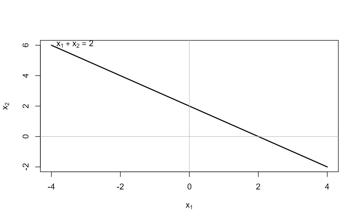
# plotEqn works for this case
plotEqn(A2, b2)
#> x[1] + x[2] = 2