High School and Beyond Data — HSB • candisc

The High School and Beyond Project was a longitudinal study of students in the U.S. carried out in 1980 by the National Center for Education Statistics. Data were collected from 58,270 high school students (28,240 seniors and 30,030 sophomores) and 1,015 secondary schools. The HSB data frame is sample of 600 observations, of unknown characteristics, originally taken from Tatsuoka (1988).

Format

A data frame with 600 observations on the following 15 variables. There is no missing data.

id: Observation id: a numeric vector
gender: a factor with levels male female
race: Race or ethnicity: a factor with levels hispanic asian african-amer white
ses: Socioeconomic status: a factor with levels low middle high
sch: School type: a factor with levels public private
prog: High school program: a factor with levels general academic vocation
locus: Locus of control: a numeric vector
concept: Self-concept: a numeric vector
mot: Motivation: a numeric vector
career: Career plan: a factor with levels clerical craftsman farmer homemaker laborer manager military operative prof1 prof2 proprietor protective sales school service technical not working
read: Standardized reading score: a numeric vector
write: Standardized writing score: a numeric vector
math: Standardized math score: a numeric vector
sci: Standardized science score: a numeric vector
ss: Standardized social science (civics) score: a numeric vector

Source

Tatsuoka, M. M. (1988). Multivariate Analysis: Techniques for Educational and Psychological Research (2nd ed.). New York: Macmillan, Appendix F, 430-442.

% Originally retrieved from: http://www.gseis.ucla.edu/courses/data/hbs6.dta

References

High School and Beyond data files: http://www.icpsr.umich.edu/icpsrweb/ICPSR/studies/7896

Examples


str(HSB)
#> 'data.frame':	600 obs. of  15 variables:
#>  $ id     : num  55 114 490 44 26 510 133 213 548 309 ...
#>  $ gender : Factor w/ 2 levels "male","female": 2 1 1 2 2 1 2 2 2 2 ...
#>  $ race   : Factor w/ 4 levels "hispanic","asian",..: 1 3 4 1 1 4 3 4 4 4 ...
#>  $ ses    : Factor w/ 3 levels "low","middle",..: 1 2 2 1 2 2 1 1 2 3 ...
#>  $ sch    : Factor w/ 2 levels "public","private": 1 1 1 1 1 1 1 1 2 1 ...
#>  $ prog   : Factor w/ 3 levels "general","academic",..: 1 2 3 3 2 3 3 1 2 1 ...
#>  $ locus  : num  -1.78 0.24 -1.28 0.22 1.12 ...
#>  $ concept: num  0.56 -0.35 0.34 -0.76 -0.74 ...
#>  $ mot    : num  1 1 0.33 1 0.67 ...
#>  $ career : Factor w/ 17 levels "clerical","craftsman",..: 9 8 9 15 15 8 14 1 10 10 ...
#>  $ read   : num  28.3 30.5 31 31 31 ...
#>  $ write  : num  46.3 35.9 35.9 41.1 41.1 ...
#>  $ math   : num  42.8 36.9 46.1 49.2 36 ...
#>  $ sci    : num  44.4 33.6 39 33.6 36.9 ...
#>  $ ss     : num  50.6 40.6 45.6 35.6 45.6 ...
# main effects model
hsb.mod <- lm( cbind(read, write, math, sci, ss) ~
    gender + race + ses + sch + prog, data=HSB)
car::Anova(hsb.mod)
#> 
#> Type II MANOVA Tests: Pillai test statistic
#>        Df test stat approx F num Df den Df    Pr(>F)    
#> gender  1   0.19207  27.8615      5    586 < 2.2e-16 ***
#> race    3   0.20268   8.5207     15   1764 < 2.2e-16 ***
#> ses     2   0.04965   2.9886     10   1174 0.0009909 ***
#> sch     1   0.01225   1.4535      5    586 0.2032987    
#> prog    2   0.21466  14.1152     10   1174 < 2.2e-16 ***
#> ---
#> Signif. codes:  0 '***' 0.001 '**' 0.01 '*' 0.05 '.' 0.1 ' ' 1

# Add some interactions
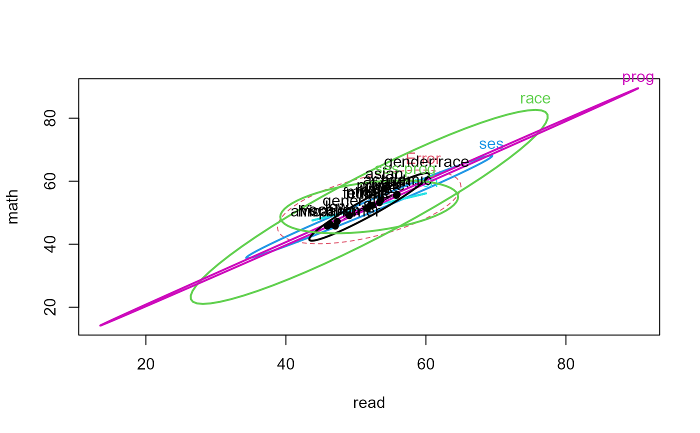
hsb.mod1 <- update(hsb.mod, . ~ . + gender:race + ses:prog)
heplot(hsb.mod1, col=palette()[c(2,1,3:6)], variables=c("read","math"))


hsb.can1 <- candisc(hsb.mod1, term="race")
heplot(hsb.can1, col=c("red", "black"))

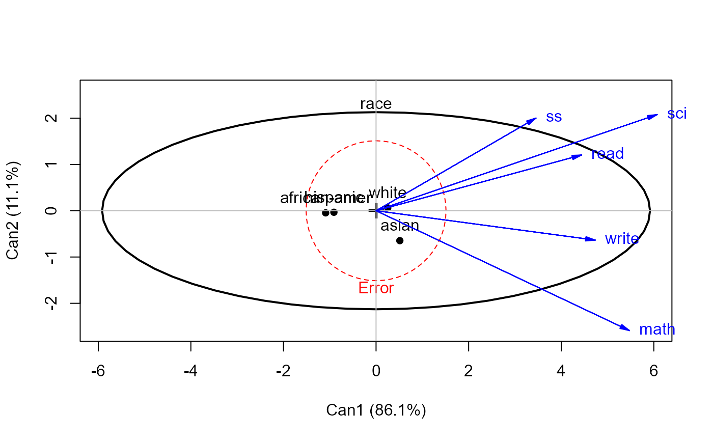#> Vector scale factor set to  6.5031 

# show canonical results for all terms
if (FALSE) { # \dontrun{
hsb.can <- candiscList(hsb.mod)
hsb.can
} # }