Three Forms of Frequency Tables for Mosaic Displays

library(ggmosaic2)
library(vcdExtra)
library(dplyr)

Introduction

Categorical data can be represented in three fundamentally different forms, each with advantages for different purposes. Understanding these forms and how to convert between them is essential for effective visualization and analysis with mosaic plots. This vignette illustrates:

The three forms of frequency tables (table form, frequency form, and case form)
Conversions between these forms
Using geom_mosaic() with each form
Comparing default shading vs. residual-based shading from loglinear models

We’ll use the classic HairEyeColor dataset throughout to demonstrate these concepts with both two-way and three-way tables.

For a comprehensive treatment of these forms and conversions, see the vcdExtra vignette by Friendly & Meyer (2016).

The Three Forms

Table Form

Table form represents categorical data as an array or table object where: - Dimensions correspond to categorical variables - Elements contain cell frequencies - Dimension names provide variable and level information

This is the most compact representation and the natural output from table() and xtabs().

# HairEyeColor is already in table form
str(HairEyeColor)
#>  'table' num [1:4, 1:4, 1:2] 32 53 10 3 11 50 10 30 10 25 ...
#>  - attr(*, "dimnames")=List of 3
#>   ..$ Hair: chr [1:4] "Black" "Brown" "Red" "Blond"
#>   ..$ Eye : chr [1:4] "Brown" "Blue" "Hazel" "Green"
#>   ..$ Sex : chr [1:2] "Male" "Female"
class(HairEyeColor)
#> [1] "table"

# Examine the 3-way table structure
HairEyeColor
#> , , Sex = Male
#> 
#>        Eye
#> Hair    Brown Blue Hazel Green
#>   Black    32   11    10     3
#>   Brown    53   50    25    15
#>   Red      10   10     7     7
#>   Blond     3   30     5     8
#> 
#> , , Sex = Female
#> 
#>        Eye
#> Hair    Brown Blue Hazel Green
#>   Black    36    9     5     2
#>   Brown    66   34    29    14
#>   Red      16    7     7     7
#>   Blond     4   64     5     8

# Total observations
sum(HairEyeColor)
#> [1] 592

The HairEyeColor dataset is a 4 × 4 × 2 contingency table with 592 observations classified by hair color, eye color, and sex.

Table form can also be displayed as a heatmap-style color table, using vcdExtra::color_table(), which shades each cell background by its frequency. This gives a quick visual sense of where the data are concentrated, as a complement to the mosaic plots introduced below – useful for readers less familiar with reading mosaic displays.

color_table(HairEyeColor, shade = "freq")

		Eye				Total
		Brown	Blue	Hazel	Green	Total
Black	Male	32	11	10	3	56
Black	Female	36	9	5	2	52
Brown	Male	53	50	25	15	143
Brown	Female	66	34	29	14	143
Red	Male	10	10	7	7	34
Red	Female	16	7	7	7	37
Blond	Male	3	30	5	8	46
Blond	Female	4	64	5	8	81
Total		220	215	93	64	592

Frequency Form

Frequency form is a data frame where: - Each row represents one cell of the contingency table - Factor columns specify the cell’s coordinates - A frequency column (typically Freq) contains the count for that cell - Total observations = sum(df$Freq)

This form is convenient for modeling and is the output from as.data.frame() applied to tables.

# Convert table to frequency form
hair_freq <- as.data.frame(HairEyeColor)
head(hair_freq, 10)
#>     Hair   Eye  Sex Freq
#> 1  Black Brown Male   32
#> 2  Brown Brown Male   53
#> 3    Red Brown Male   10
#> 4  Blond Brown Male    3
#> 5  Black  Blue Male   11
#> 6  Brown  Blue Male   50
#> 7    Red  Blue Male   10
#> 8  Blond  Blue Male   30
#> 9  Black Hazel Male   10
#> 10 Brown Hazel Male   25
nrow(hair_freq)  # 32 cells in the 4 × 4 × 2 table
#> [1] 32

# Verify totals match
sum(hair_freq$Freq)
#> [1] 592

Frequency form is ideal for: - Input to modeling functions (glm(), loglm(), etc.) - Filtering specific cells or combinations - Adding derived variables - Use with ggplot2 via the weight aesthetic

Case Form

Case form represents data as: - Each row is one individual observation - Factor columns contain the variable values for that individual - No frequency column needed - Total observations = nrow(df)

This is the “raw data” format and most intuitive for those familiar with data collection.

# Convert frequency form to case form using vcdExtra::expand.dft()
hair_case <- expand.dft(hair_freq, freq = "Freq")
head(hair_case, 10)
#>     Hair   Eye  Sex
#> 1  Black Brown Male
#> 2  Black Brown Male
#> 3  Black Brown Male
#> 4  Black Brown Male
#> 5  Black Brown Male
#> 6  Black Brown Male
#> 7  Black Brown Male
#> 8  Black Brown Male
#> 9  Black Brown Male
#> 10 Black Brown Male
nrow(hair_case)  # 592 individual observations
#> [1] 592

# Structure
str(hair_case)
#> 'data.frame':    592 obs. of  3 variables:
#>  $ Hair: chr  "Black" "Black" "Black" "Black" ...
#>  $ Eye : chr  "Brown" "Brown" "Brown" "Brown" ...
#>  $ Sex : chr  "Male" "Male" "Male" "Male" ...

Case form is most natural when: - Working with individual-level data - Each observation represents one subject - No need to aggregate

Converting Between Forms

The table below summarizes conversion functions:

From → To	Table	Frequency	Case
Table	—	`as.data.frame()`	`expand.dft()`
Frequency	`xtabs(Freq ~ ...)`	—	`expand.dft()`
Case	`table()`, `xtabs()`	`count()`, `xtabs()`	—

Note: These conversions are clearly untidy and hard to remember which to use. They have now been implemented in a collection of vcdExtra::as_*() functions which take whatever you give it and return the desired form.

Examples

# Case → Frequency (count occurrences)
hair_case |>
  count(Hair, Eye, Sex, name = "Freq") |>
  head()
#>    Hair   Eye    Sex Freq
#> 1 Black  Blue Female    9
#> 2 Black  Blue   Male   11
#> 3 Black Brown Female   36
#> 4 Black Brown   Male   32
#> 5 Black Green Female    2
#> 6 Black Green   Male    3

# Frequency → Table
hair_table <- xtabs(Freq ~ Hair + Eye + Sex, data = hair_freq)
identical(hair_table, HairEyeColor)
#> [1] FALSE

# Table → Frequency (already shown)
# Frequency → Case (already shown)

Using Each Form with `geom_mosaic()`

Working with the Three-Way Table: Hair × Eye × Sex

Let’s demonstrate how to use each of the three forms with geom_mosaic() using the full HairEyeColor dataset.

# From frequency form (most common)
ggplot(data = hair_freq,
       aes(weight = Freq, x = product(Hair, Eye, Sex), fill = Eye)) +
  geom_mosaic() +
  labs(title = "Three-Way Mosaic: Hair × Eye × Sex",
       subtitle = "Frequency form with weight aesthetic")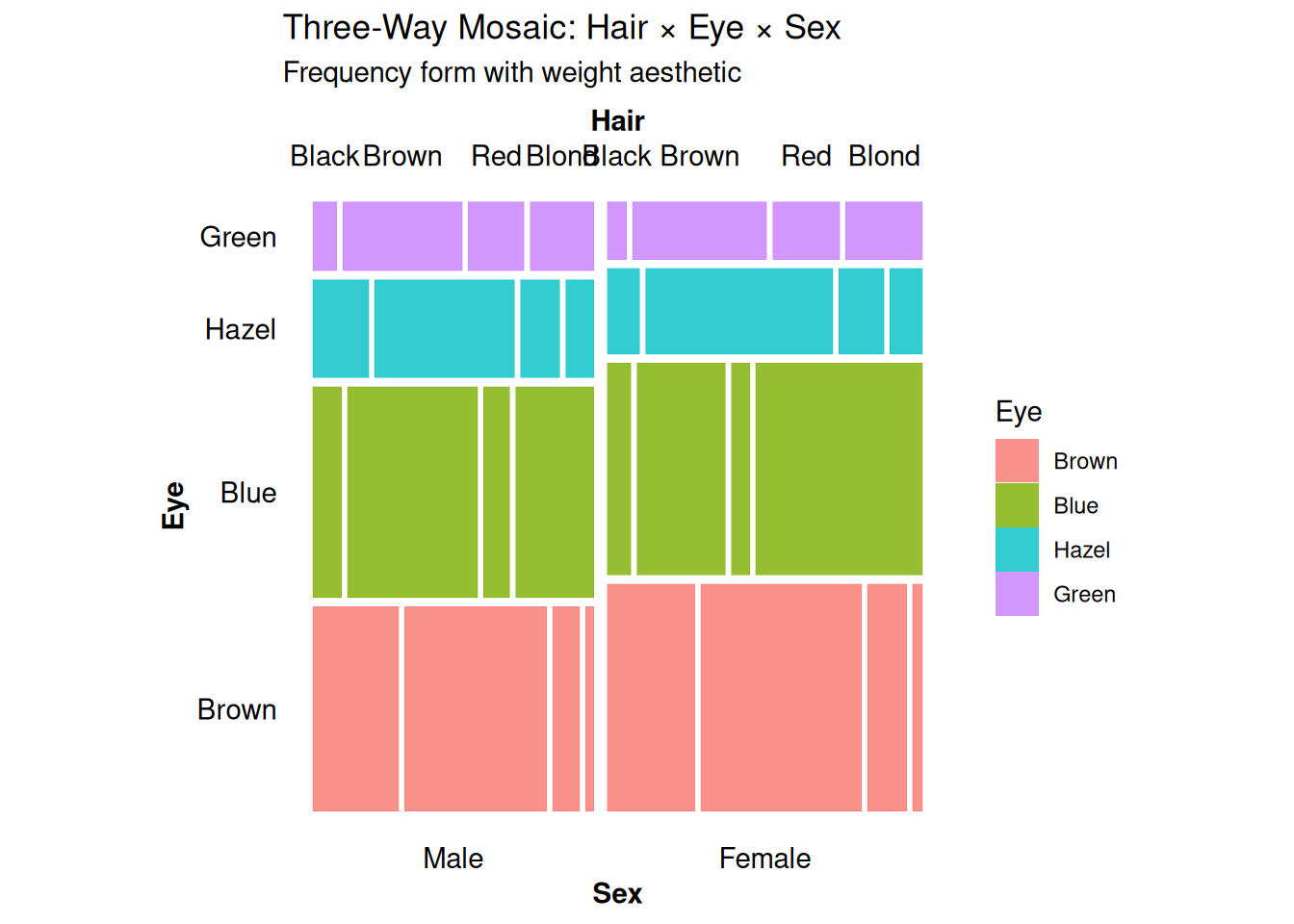

# From case form
ggplot(data = hair_case,
       aes(x = product(Hair, Eye, Sex), fill = Eye)) +
  geom_mosaic() +
  labs(title = "Three-Way Mosaic: Hair × Eye × Sex",
       subtitle = "Case form without weight")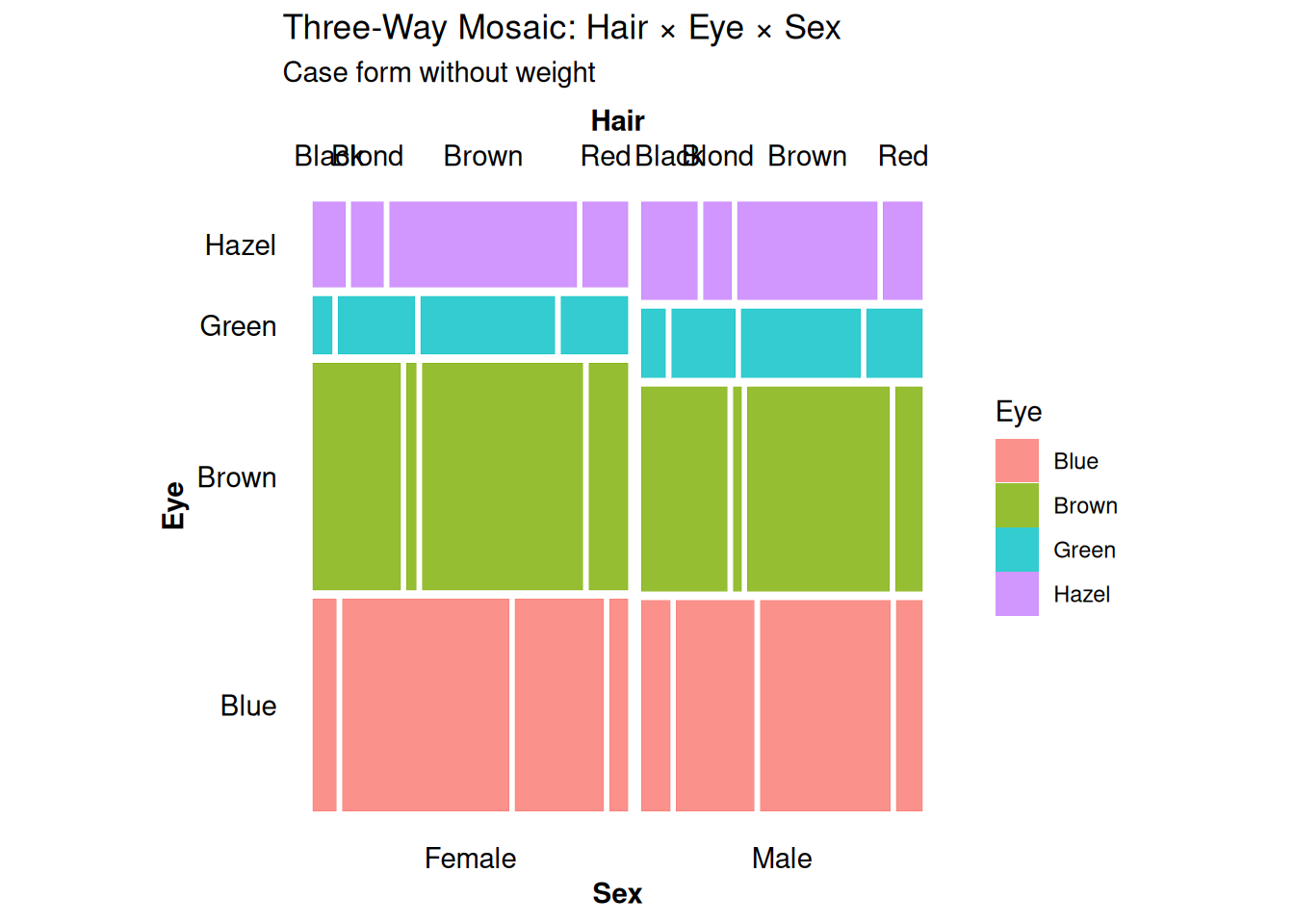

Both forms produce identical plots. The key difference: - Frequency form: Use weight = Freq in the aesthetic - Case form: No weight needed (each row counts as 1)

Note: Table form data must first be converted to frequency form using as.data.frame() before use with geom_mosaic().

Using Conditioning Variables

The conds aesthetic allows you to condition on one or more variables:

# Condition on Sex
ggplot(data = hair_freq,
       aes(weight = Freq,
           x = product(Hair, Eye),
           conds = product(Sex),
           fill = Eye)) +
  geom_mosaic() +
  labs(title = "Hair × Eye | Sex",
       subtitle = "Conditioned on Sex")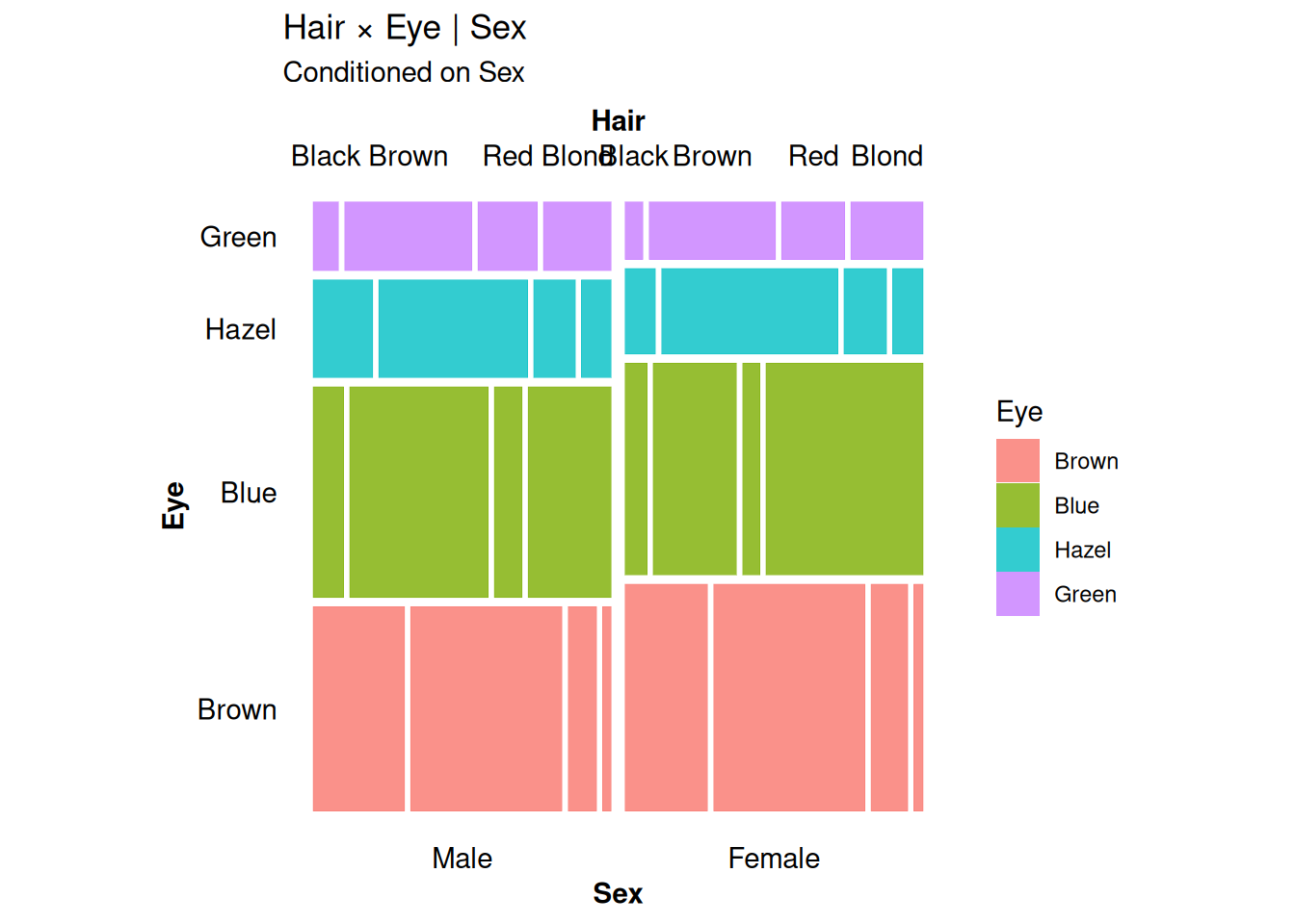

Default Shading vs. Residual-Based Shading

One of the most powerful features of mosaic plots is residual-based shading, which highlights deviations from a statistical model. This allows us to see not just the data, but whether patterns are statistically meaningful.

Default Shading

By default, geom_mosaic() uses the fill aesthetic to color tiles, typically showing one of the categorical variables:

ggplot(data = hair_freq,
       aes(weight = Freq, x = product(Hair, Eye), fill = Eye)) +
  geom_mosaic() +
  labs(title = "Hair × Eye Color: Default Shading",
       subtitle = "Fill shows Eye color levels")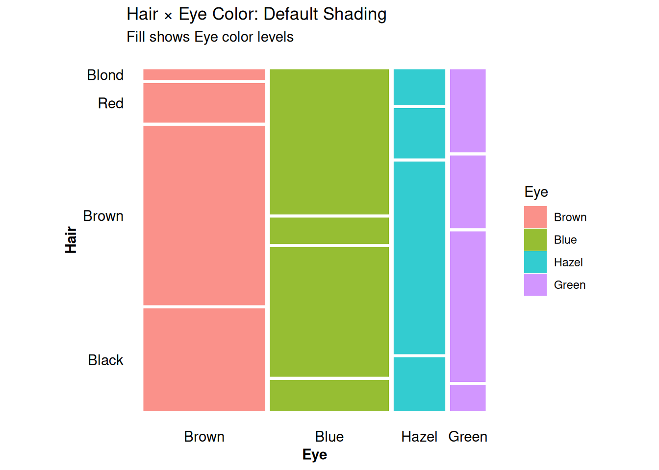

This clearly shows the marginal and conditional distributions, but doesn’t tell us whether associations are statistically significant.

Residual-Based Shading

Residual-based shading fits a loglinear model to the data and colors tiles according to Pearson residuals:

$r_{ij} = \frac{\text{observed}_{ij} - \text{expected}_{ij}}{\sqrt{\text{expected}_{ij}}}$

where “expected” frequencies come from the fitted model.

Blue tiles: Observed > Expected (positive association)
Red tiles: Observed < Expected (negative association)
Intensity: Magnitude of the residual
|r| > 2: Statistically significant at approximately α = 0.05

Independence Model for Two-Way Table

For a two-way table, we can visualize just Hair and Eye color. The most common model is independence (main effects only):

ggplot(data = hair_freq,
       aes(weight = Freq, x = product(Hair, Eye))) +
  geom_mosaic(expected = "independence") +
  scale_fill_residual() +
  labs(title = "Hair × Eye Color: Independence Model",
       subtitle = "Blue = more than expected, Red = fewer than expected")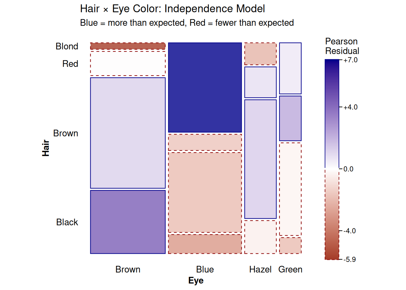

The residual shading reveals: - Blue tiles (positive residuals): Black hair with brown eyes, blond hair with blue eyes occur more frequently than independence would predict - Red tiles (negative residuals): Black hair with blue eyes, blond hair with brown eyes occur less frequently - This indicates a significant association between hair and eye color

Adding Cell Values

We can display the actual residual values in each cell using geom_mosaic_text():

ggplot(data = hair_freq,
       aes(weight = Freq, x = product(Hair, Eye))) +
  mosaic_settings(expected = "independence") +
  geom_mosaic() +
  scale_fill_residual() +
  geom_mosaic_text(display_values = "residual",
                   format_digits = 1,
                   size = 3.5,
                   colour = "black") +
  labs(title = "Hair × Eye Independence Model with Residual Values",
       subtitle = "Numbers show Pearson residuals")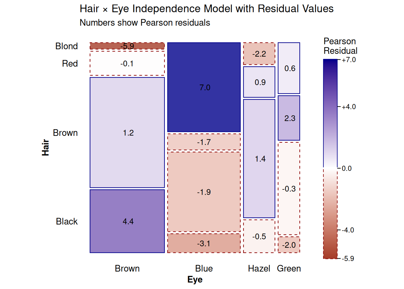

Values greater than 2 in absolute value indicate significant departures from independence.

Independence Model for Three-Way Table

For the three-way table, the independence model tests whether all three variables are mutually independent:

ggplot(data = hair_freq,
       aes(weight = Freq, x = product(Hair, Eye, Sex))) +
  geom_mosaic(expected = "independence") +
  scale_fill_residual() +
  labs(title = "Hair × Eye × Sex: Complete Independence",
       subtitle = "Model: ~ Hair + Eye + Sex (no interactions)")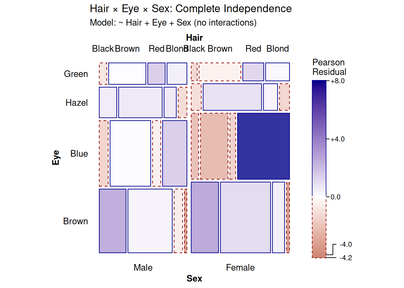

Custom Models

You can specify custom loglinear models using formula syntax. For example, testing whether the Hair-Eye association differs by Sex:

# Model: Hair and Eye are associated, but independent of Sex
ggplot(data = hair_freq,
       aes(weight = Freq, x = product(Hair, Eye, Sex))) +
  geom_mosaic(expected = ~ Hair * Eye + Sex) +
  scale_fill_residual() +
  labs(title = "Model: (Hair × Eye) Independent of Sex",
       subtitle = "~ Hair * Eye + Sex")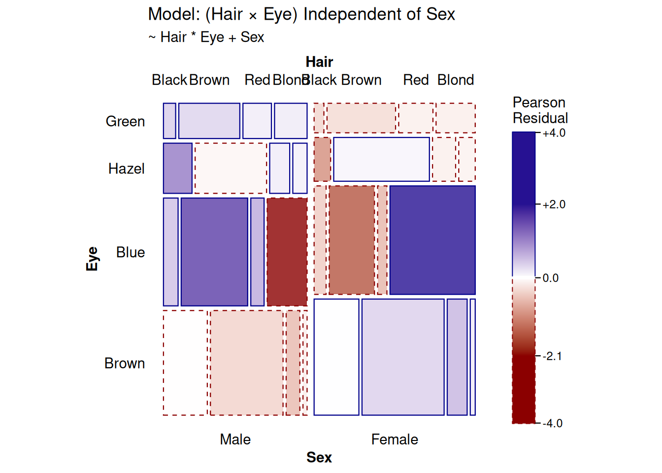

Residuals close to zero suggest this model fits reasonably well—the Hair-Eye association is similar for males and females.

Comparing Observed and Expected

We can also display the expected counts under a model:

ggplot(data = hair_freq,
       aes(weight = Freq, x = product(Hair, Eye))) +
  mosaic_settings(expected = "independence") +
  geom_mosaic() +
  scale_fill_residual() +
  geom_mosaic_text(display_values = "expected",
                   format_digits = 1,
                   size = 3.5,
                   colour = "black") +
  labs(title = "Expected Frequencies Under Independence",
       subtitle = "Compare with observed to see associations")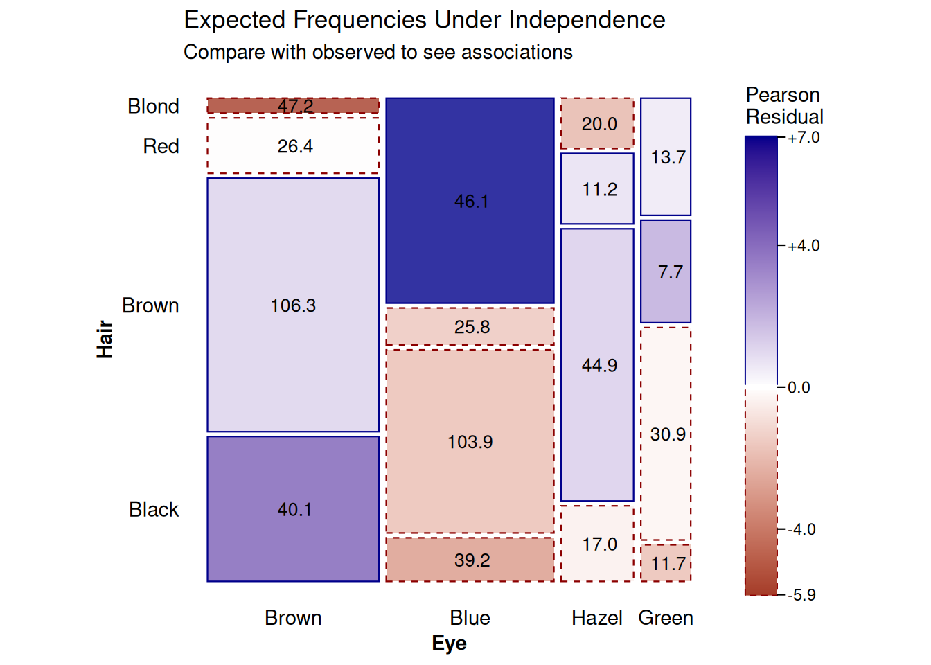

And the observed counts:

ggplot(data = hair_freq,
       aes(weight = Freq, x = product(Hair, Eye))) +
  geom_mosaic(aes(fill = Eye)) +
  geom_mosaic_text(display_values = "observed",
                   format_digits = 0,
                   size = 3.5,
                   colour = "white") +
  labs(title = "Observed Frequencies",
       subtitle = "Actual counts in each cell")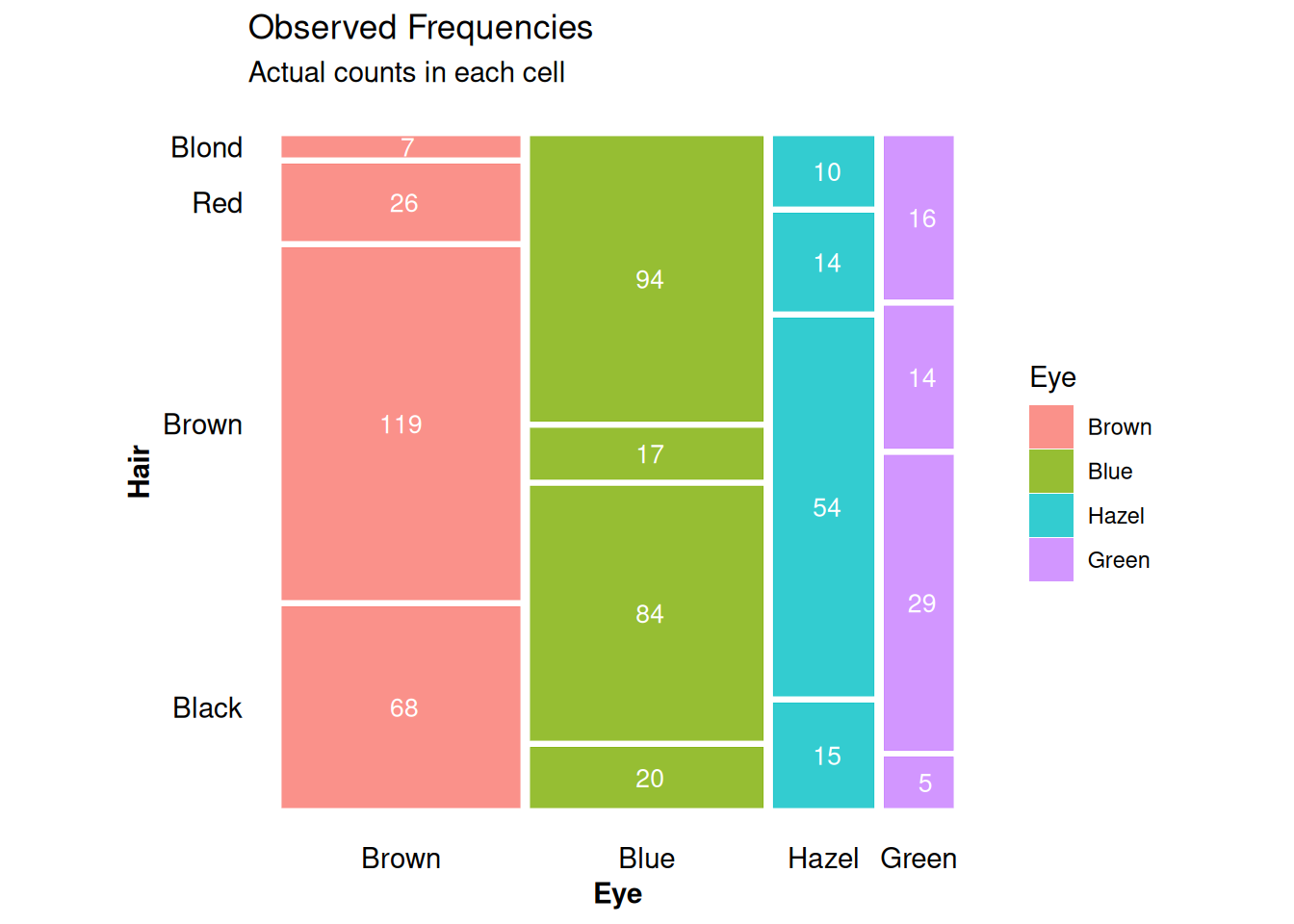

Summary

Key Takeaways

Three forms of frequency data serve different purposes:
- Table form: Compact, ideal for arrays and mathematical operations
- Frequency form: Versatile, works well with modeling and ggplot2
- Case form: Intuitive, represents raw individual-level data
Converting between forms is straightforward:
- Use as.data.frame() for table → frequency
- Use expand.dft() for frequency → case
- Use xtabs() or table() for case/frequency → table
Using with geom_mosaic():
- Table/frequency forms require weight = Freq
- Case form works directly (no weight)
- All forms produce identical visualizations
Two types of shading:
- Default: Uses fill aesthetic to show variable levels
- Residual-based: Uses expected parameter to fit models and shade by Pearson residuals
Residual shading is powerful for:
- Identifying statistically significant associations
- Testing specific hypotheses about independence
- Comparing observed patterns to theoretical models

Recommendations

For visualization: Frequency form with weight aesthetic is most flexible
For modeling: Frequency form works with glm(), loglm(), etc.
For raw data: Case form is most intuitive
For residual plots: Always use scale_fill_residual() and consider adding geom_mosaic_text() with display_values = "residual"

References

Friendly, M. (1994). “Mosaic Displays for Multi-Way Contingency Tables.” Journal of the American Statistical Association, 89(425), 190-200.
Friendly, M., & Meyer, D. (2016). Discrete Data Analysis with R. Chapman and Hall/CRC.
Meyer, D., Zeileis, A., & Hornik, K. (2006). “The Strucplot Framework: Visualizing Multi-way Contingency Tables with vcd.” Journal of Statistical Software, 17(3), 1-48.
Zeileis, A., Meyer, D., & Hornik, K. (2007). “Residual-based Shadings for Visualizing (Conditional) Independence.” Journal of Computational and Graphical Statistics, 16(3), 507-525.

Session Info

sessionInfo()
#> R version 4.6.1 (2026-06-24)
#> Platform: x86_64-pc-linux-gnu
#> Running under: Ubuntu 24.04.5 LTS
#> 
#> Matrix products: default
#> BLAS:   /usr/lib/x86_64-linux-gnu/openblas-pthread/libblas.so.3 
#> LAPACK: /usr/lib/x86_64-linux-gnu/openblas-pthread/libopenblasp-r0.3.26.so;  LAPACK version 3.12.0
#> 
#> locale:
#>  [1] LC_CTYPE=C.UTF-8       LC_NUMERIC=C           LC_TIME=C.UTF-8       
#>  [4] LC_COLLATE=C.UTF-8     LC_MONETARY=C.UTF-8    LC_MESSAGES=C.UTF-8   
#>  [7] LC_PAPER=C.UTF-8       LC_NAME=C              LC_ADDRESS=C          
#> [10] LC_TELEPHONE=C         LC_MEASUREMENT=C.UTF-8 LC_IDENTIFICATION=C   
#> 
#> time zone: UTC
#> tzcode source: system (glibc)
#> 
#> attached base packages:
#> [1] grid      stats     graphics  grDevices utils     datasets  methods  
#> [8] base     
#> 
#> other attached packages:
#> [1] dplyr_1.2.1     vcdExtra_0.9.8  gnm_1.1-5       vcd_1.4-14     
#> [5] ggmosaic2_0.5.1 ggplot2_4.0.3  
#> 
#> loaded via a namespace (and not attached):
#>  [1] gtable_0.3.6        xfun_0.60           bslib_0.12.0       
#>  [4] htmlwidgets_1.6.4   websocket_1.4.4     ggrepel_0.9.8      
#>  [7] processx_3.9.0      lattice_0.22-9      vctrs_0.7.3        
#> [10] tools_4.6.1         ps_1.9.3            generics_0.1.4     
#> [13] tibble_3.3.1        ca_0.72             pkgconfig_2.0.3    
#> [16] Matrix_1.7-5        data.table_1.18.6.1 RColorBrewer_1.1-3 
#> [19] S7_0.2.2            desc_1.4.3          gt_1.3.0           
#> [22] lifecycle_1.0.5     compiler_4.6.1      farver_2.1.2       
#> [25] textshaping_1.0.5   chromote_0.5.1      htmltools_0.5.9    
#> [28] sass_0.4.10         yaml_2.3.12         plotly_4.12.1      
#> [31] pillar_1.11.1       pkgdown_2.2.1       later_1.4.8        
#> [34] jquerylib_0.1.4     tidyr_1.3.2         MASS_7.3-65        
#> [37] cachem_1.1.0        webshot2_0.1.2      tidyselect_1.2.1   
#> [40] digest_0.6.39       purrr_1.2.2         qvcalc_1.0.4       
#> [43] forcats_1.0.1       fastmap_1.2.0       colorspace_2.1-3   
#> [46] cli_3.6.6           magrittr_2.0.5      productplots_0.1.2 
#> [49] relimp_1.0-5        withr_3.0.3         scales_1.4.0       
#> [52] promises_1.5.0      rmarkdown_2.32      httr_1.4.9         
#> [55] otel_0.2.0          nnet_7.3-20         ragg_1.5.2         
#> [58] zoo_1.9-0           evaluate_1.0.5      knitr_1.52         
#> [61] lmtest_0.9-40       viridisLite_0.4.3   rlang_1.3.0        
#> [64] Rcpp_1.1.2          glue_1.8.1          xml2_1.6.0         
#> [67] jsonlite_2.0.0      R6_2.6.1            plyr_1.8.9         
#> [70] systemfonts_1.3.2   fs_2.1.0

Michael Friendly

2026-09-16

Introduction

The Three Forms

Table Form

Frequency Form

Case Form

Converting Between Forms

Examples

Using Each Form with `geom_mosaic()`

Working with the Three-Way Table: Hair × Eye × Sex

Using Conditioning Variables

Default Shading vs. Residual-Based Shading

Default Shading

Residual-Based Shading

Independence Model for Two-Way Table

Adding Cell Values

Independence Model for Three-Way Table

Custom Models

Comparing Observed and Expected

Summary

Key Takeaways

Recommendations

References

Session Info

Three Forms of Frequency Tables for Mosaic Displays

Michael Friendly

2026-09-16

Introduction

The Three Forms

Table Form

Frequency Form

Case Form

Converting Between Forms

Examples

Using Each Form with geom_mosaic()

Working with the Three-Way Table: Hair × Eye × Sex

Using Conditioning Variables

Default Shading vs. Residual-Based Shading

Default Shading

Residual-Based Shading

Independence Model for Two-Way Table

Adding Cell Values

Independence Model for Three-Way Table

Custom Models

Comparing Observed and Expected

Summary

Key Takeaways

Recommendations

References

Session Info

Using Each Form with `geom_mosaic()`