Introducing ggmosaic2: an enhanced ggmosaic

Gavin Klorfine

2026-09-16

library(ggmosaic2)

With ggmosaic being taken off of CRAN and appearing unmaintained (PRs and issues not receiving responses as well as minimal commit activity on the repository), there was a need to bring mosaic plots back to the ggplot2 framework. In addition to fixing outstanding issues, we (the new authors) also wanted to improve upon the existing package, as several aspects of ggmosaics were inferior and/or limited when compared to mosaics produced by vcd and vcdExtra.

This vignette describes the many additions and changes made to ggmosaic that make up the initial release of ggmosaic2. The most important of these changes, is the introduction of residual shading, to show the pattern of association in a frequency table in relation to some loglinear model. This is described in its own vignette ggmosaic and Loglinear Models.

Basic Appearance

A few things were done to alter the basic appearance of mosaics, both with and without the use of theme_mosaic():

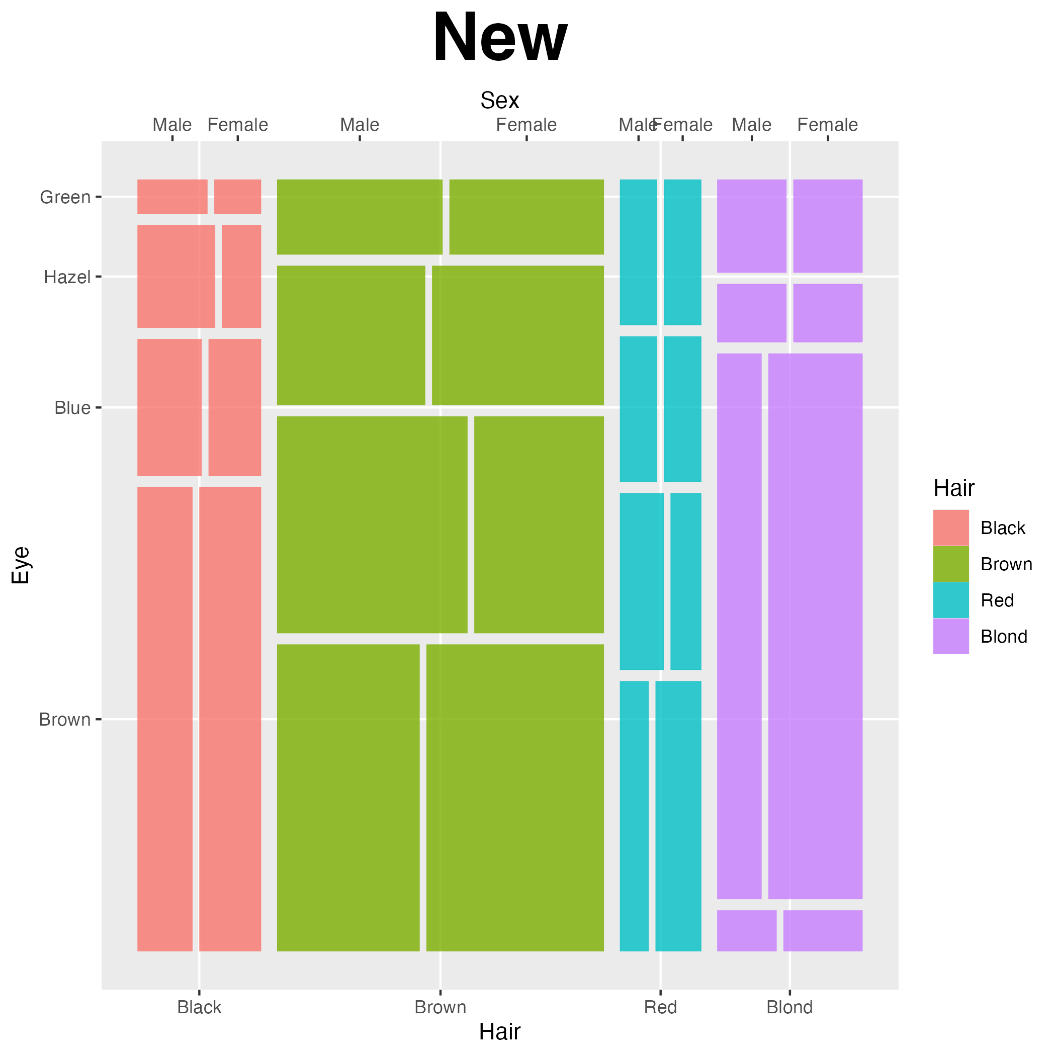
Utilizing the top and right axes

When three or more variables are used, the top (three or more variables) and right (four or more variables) axes will now be utilized. The figures compare the historical haleyjeppson/ggmosaic output (Old) with friendly/ggmosaic2 (New);

The current ggmosaic2 syntax below declares its aesthetics globally:

HairEyeColor |>
  as.data.frame() |>
  ggplot(aes(x = product(Sex, Eye, Hair), fill = Hair, weight = Freq)) +
    geom_mosaic()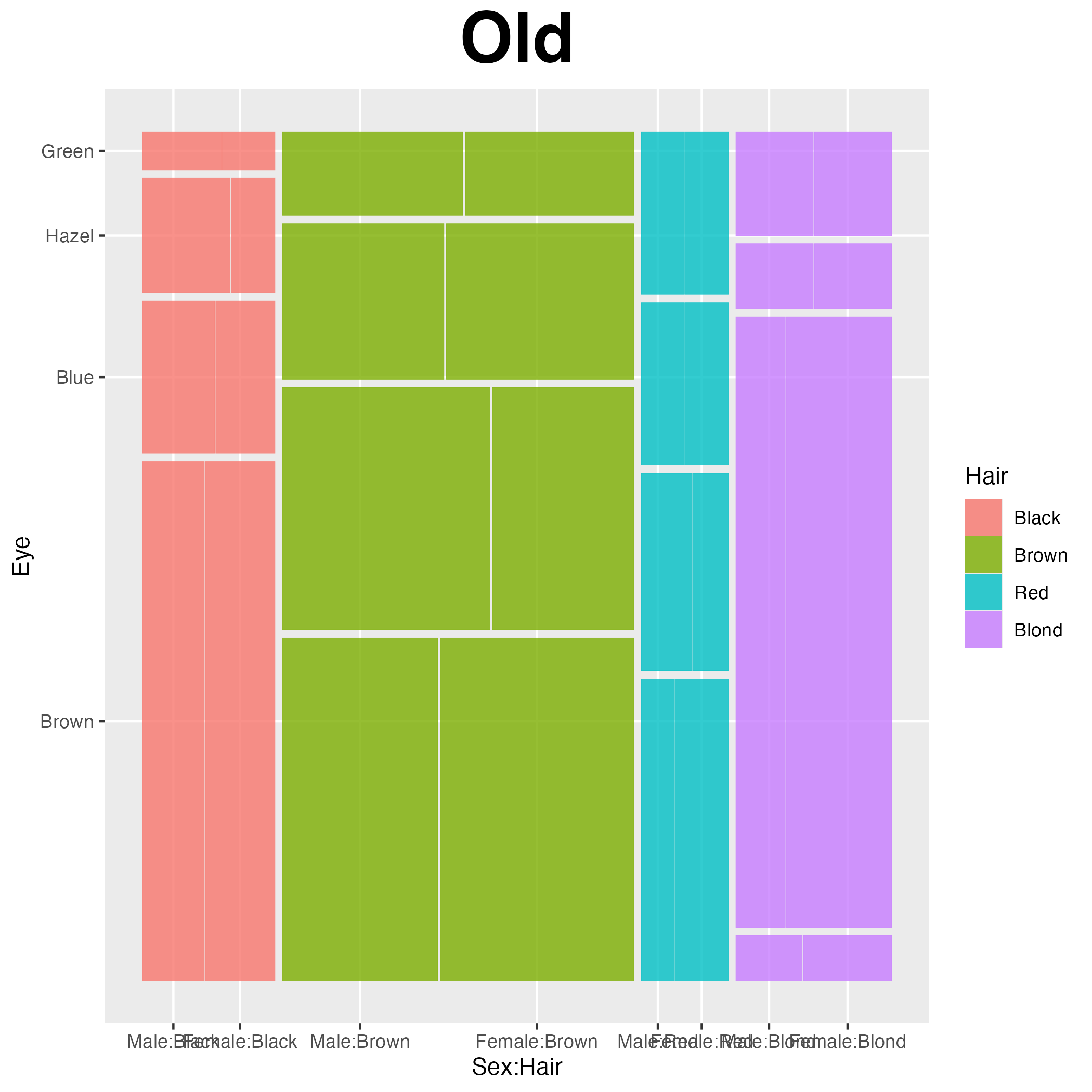

theme_mosaic()

As with other ggplot2 extensions, themes set the general look-and-feel of the plot such as the color of the background, gridlines, the size and color of fonts. theme_mosaic() provides access to the regular ggplot2 theme, but: removes any background, axes ticks, most of the gridlines, and ensures an aspect ratio of 1 for better viewing of the mosaics. This theme also applies a bold face to axes labels and allows for the convenient rotation of category labels to avoid overlap.

With theme_mosaic() applied to the above:

HairEyeColor |>
  as.data.frame() |>
  ggplot(aes(x = product(Sex, Eye, Hair), fill = Hair, weight = Freq)) +
    geom_mosaic() +
    theme_mosaic(base_size = 12)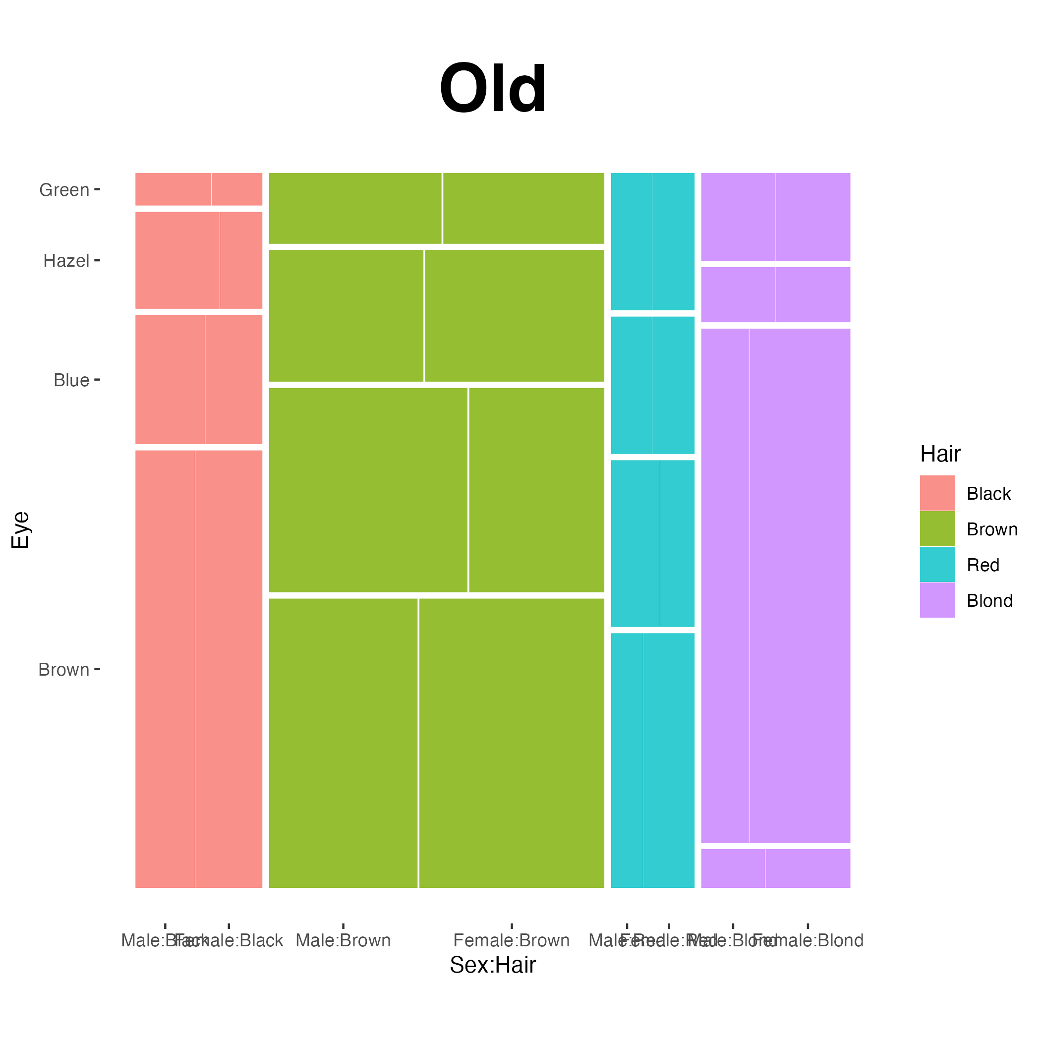

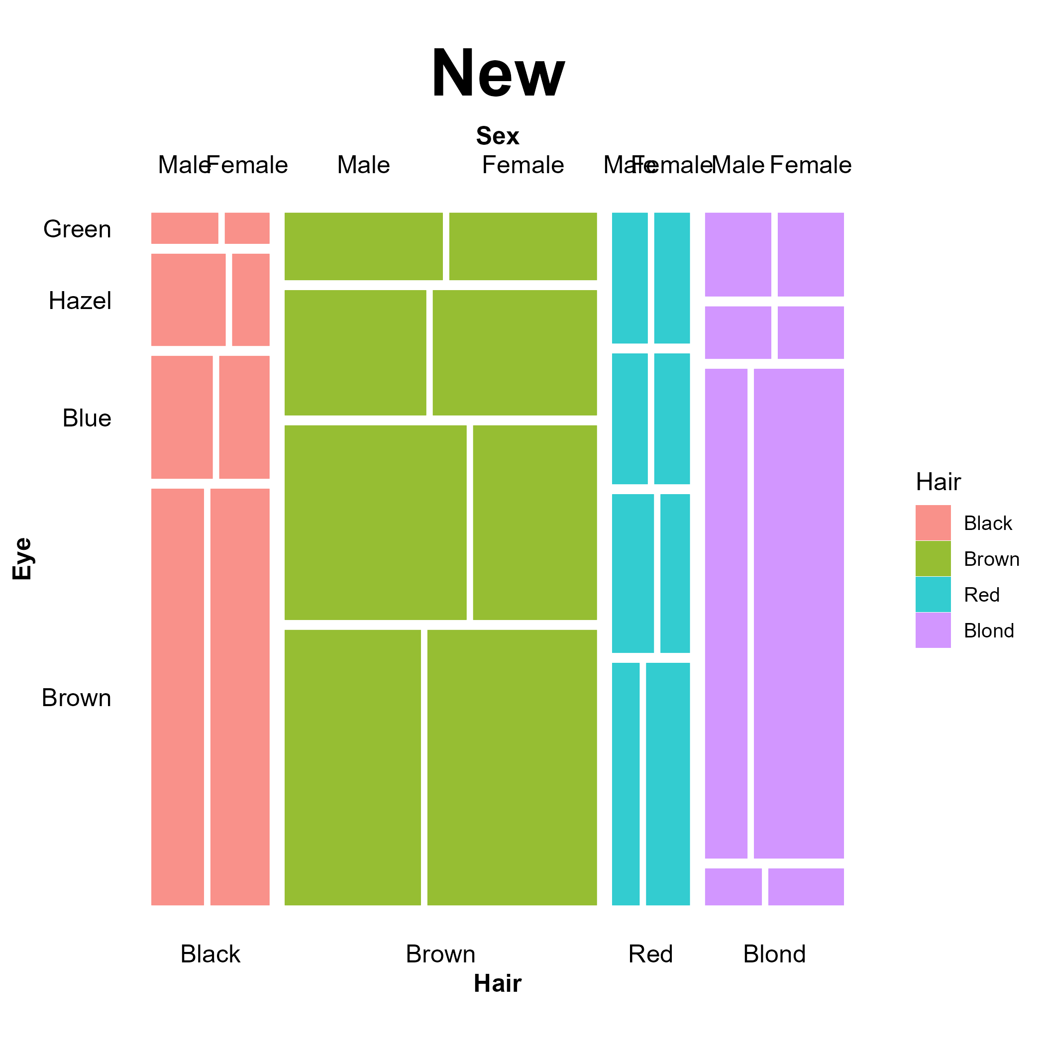
Axis labels had a bold face applied to be consistent with mosaics made using vcd and vcdExtra. Axis ticks were removed, as they are unnecessary for mosaic displays.

New to theme_mosaic() is a convenience argument rot_labels that can rotate category labels to a user-specified angle (in degrees):

HairEyeColor |>
  as.data.frame() |>
  ggplot(aes(x = product(Sex, Eye, Hair), fill = Hair, weight = Freq)) +
    geom_mosaic() +
    theme_mosaic(rot_labels = 30, base_size = 14)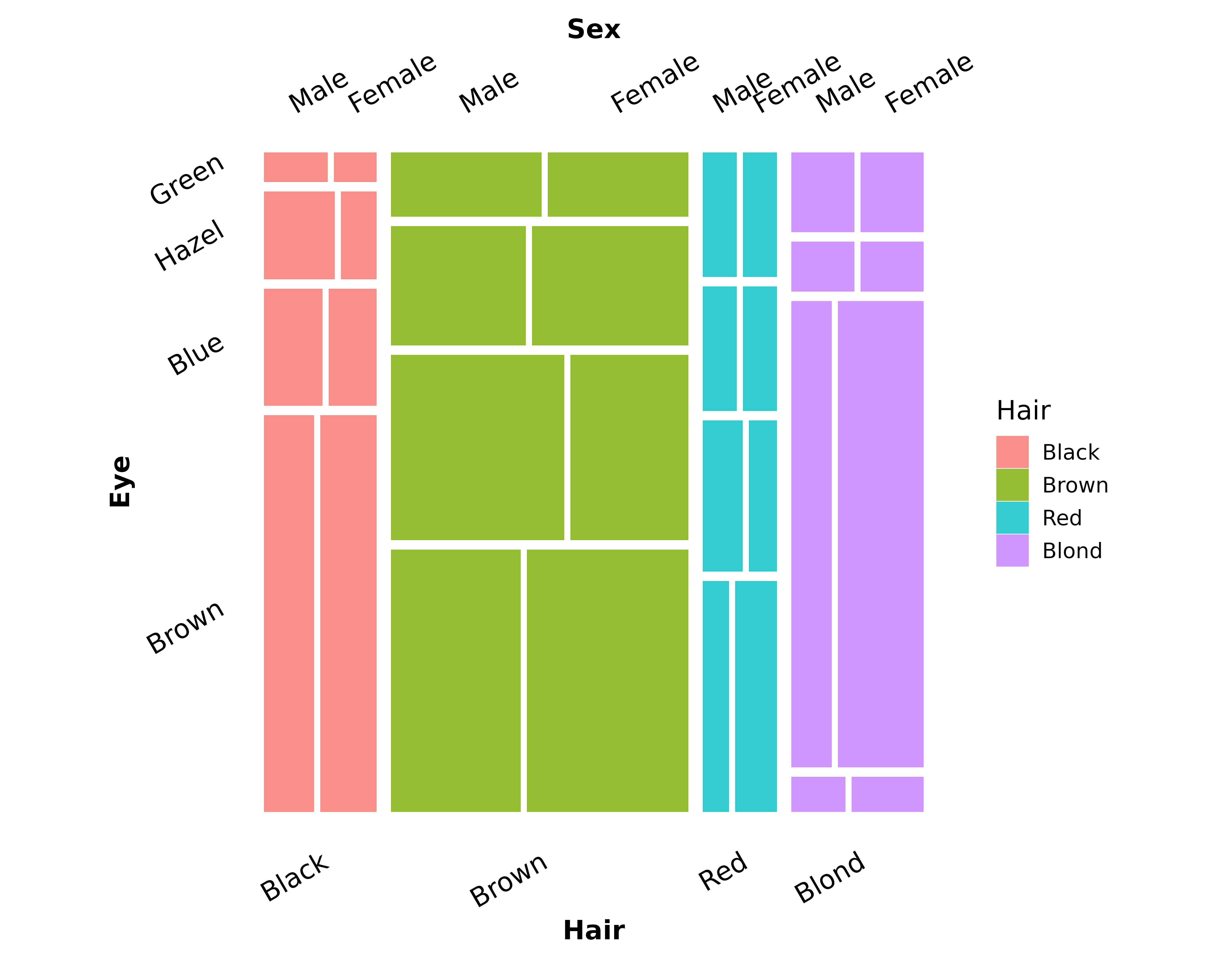

Spacing of cells

You might already have noticed that the innermost spacing of cells in mosaic displays has been increased in ggmosaic2. This is a perceptual feature of mosaic displays (Friendly, 1994): wider gaps at the first splits make it easier and compare to see the frequencies of categories at different dimensions of the table in the order the mosaic is divided.

Re-using an example from “Utilizing the top and right axes,” differentiating between cells is now easier:

HairEyeColor |>
  as.data.frame() |>
  ggplot(aes(x = product(Sex, Eye, Hair), fill = Hair, weight = Freq)) +
    geom_mosaic() +
    theme_mosaic()

In the old ggmosaic, increasing the offset argument of geom_mosaic() would not remedy this issue to a satisfying degree. ggmosaic2 solves this by implementing a spacing scheme similar to vcd:

$$\text{gap}_j = \text{offset} \times 1.5^{d - j}$$

where $d$ is the number of splits and $j = 1$ is the innermost split. offset remains at a default of .01.

Faceting is Fixed

The old ggmosaic had an issue where facet labels would not be independently generated per panel:

HairEyeColor |>
  as.data.frame() |>
  ggplot(aes(x = product(Eye, Hair), fill = Hair, weight = Freq)) +
  geom_mosaic() +
  theme_mosaic() +
  facet_grid(. ~ Sex)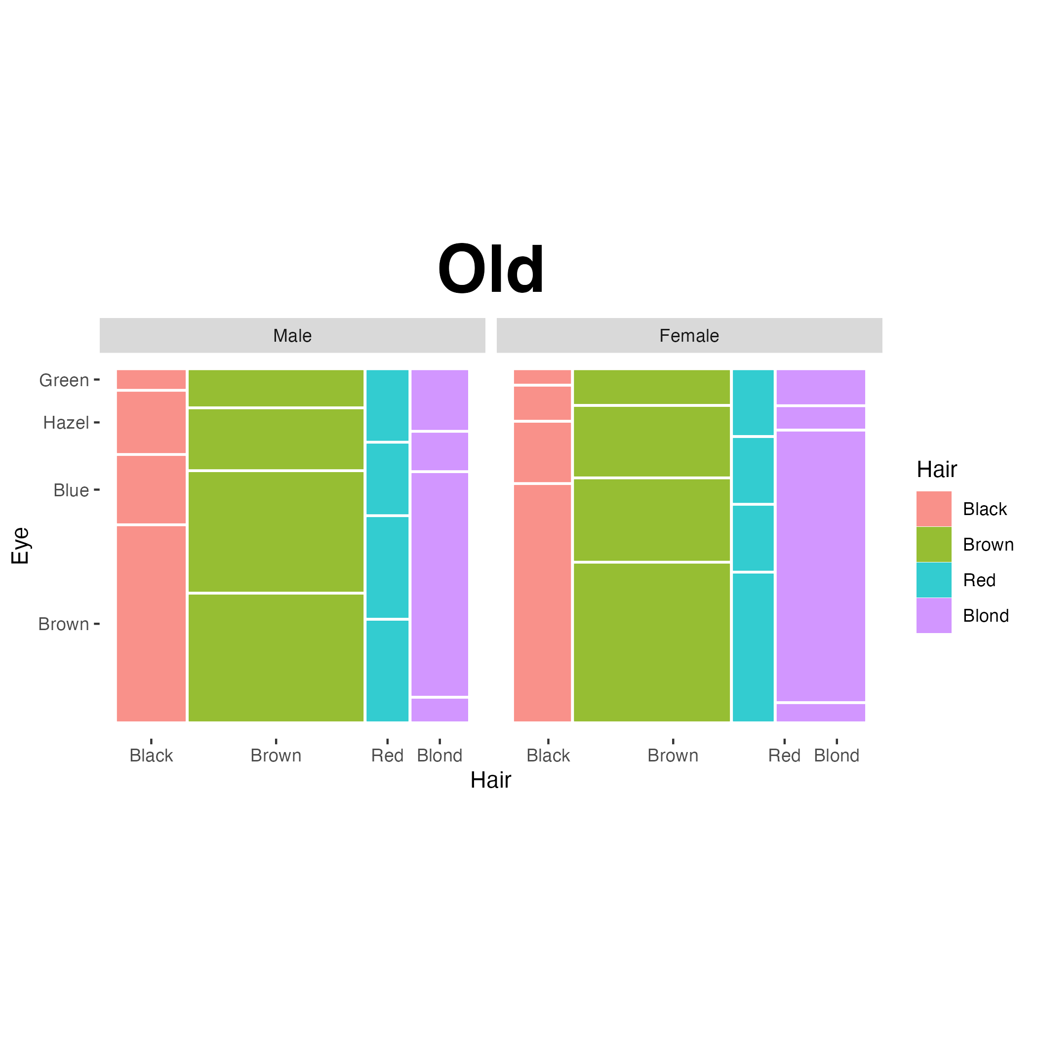

The new function facet_mosaic_grid() corrects this behavior, generating labels per facet:

HairEyeColor |>
  as.data.frame() |>
  ggplot(aes(x = product(Eye, Hair), fill = Hair, weight = Freq)) +
  geom_mosaic() +
  theme_mosaic() +
  facet_mosaic_grid(. ~ Sex)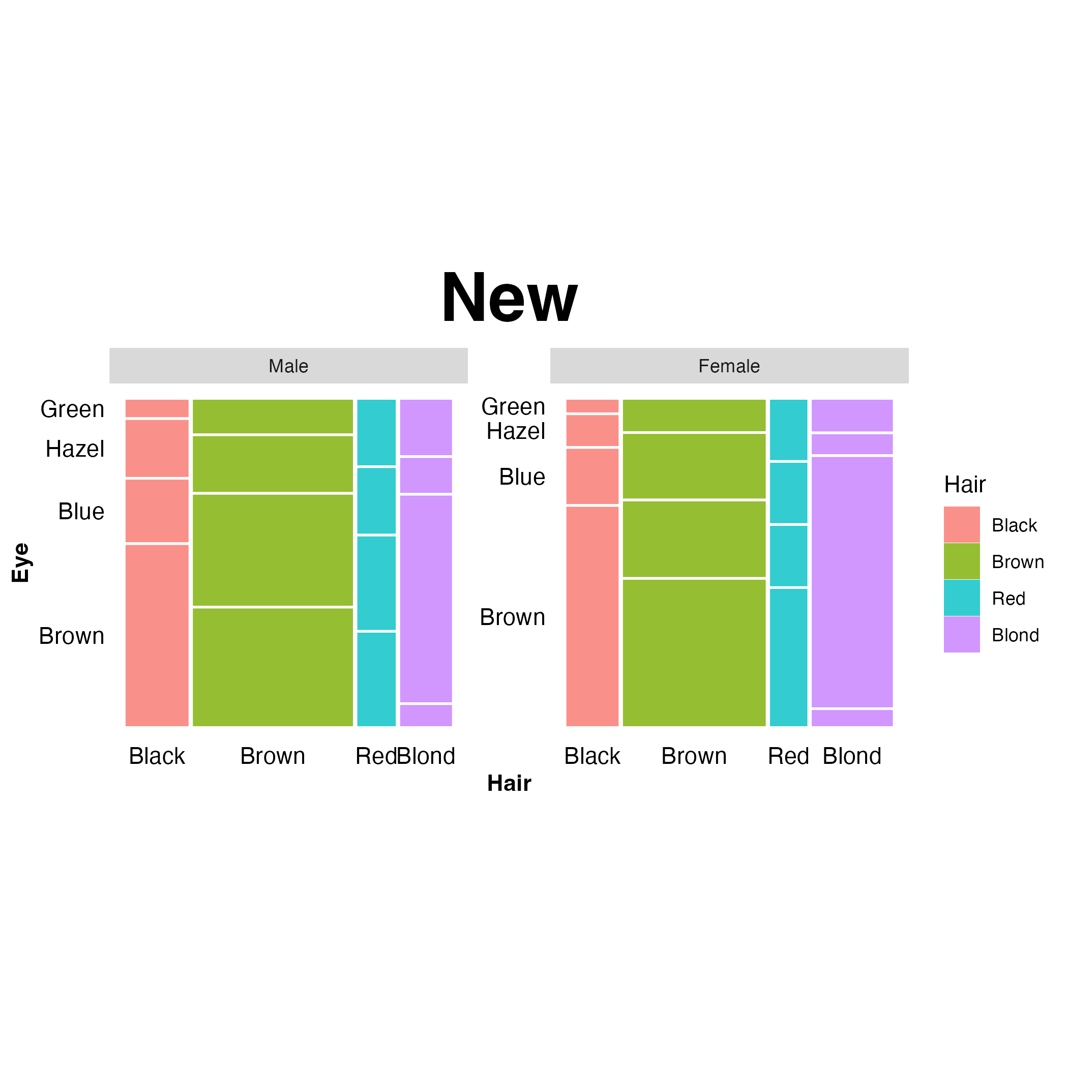

Residual-Based Shading

As stated, this portion of the vignette will be covered in minimal detail, with more information found in ggmosaic and Loglinear Models.

To apply residual-based shading to the HairEyeColor example, we will need to supply the expected argument of geom_mosaic() with a model. Let’s use the model of independence. We will also need to use scale_fill_residual() instead of the fill argument of geom_mosaic():

HairEyeColor |>
  as.data.frame() |>
  ggplot(aes(x = product(Sex, Eye, Hair), weight = Freq)) +
  geom_mosaic(expected = "independence") +
  scale_fill_residual() +
  theme_mosaic(rot_labels = 30)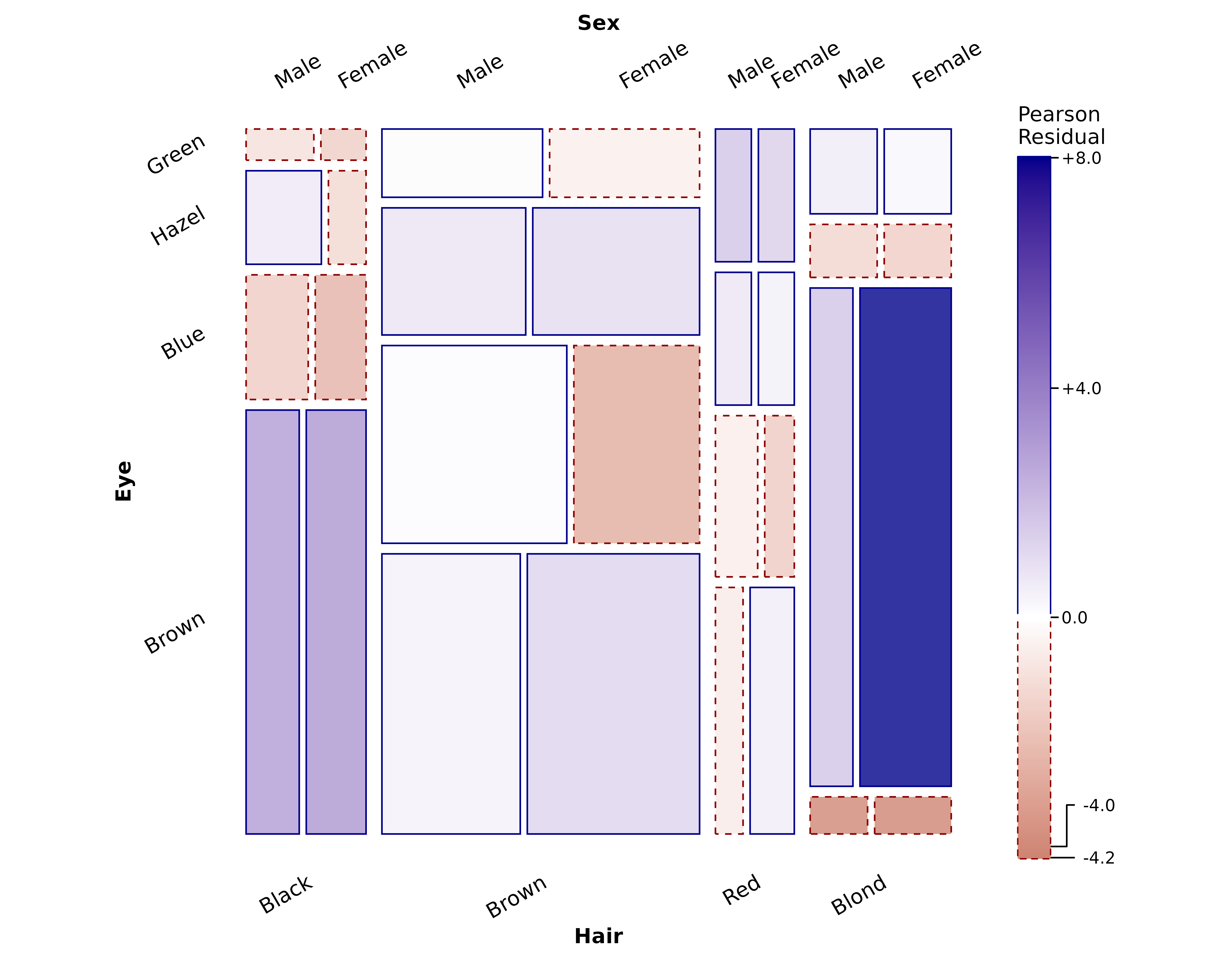

For a shading scheme that accentuates residuals $\geq \pm4$ (similar to the default in vcd), you can use the limits argument of scale_fill_residual():

HairEyeColor |>
  as.data.frame() |>
  ggplot(aes(x = product(Sex, Eye, Hair), weight = Freq)) +
  geom_mosaic(expected = "independence") +
  scale_fill_residual(limits = c(-4,4)) +
  theme_mosaic(rot_labels = 30)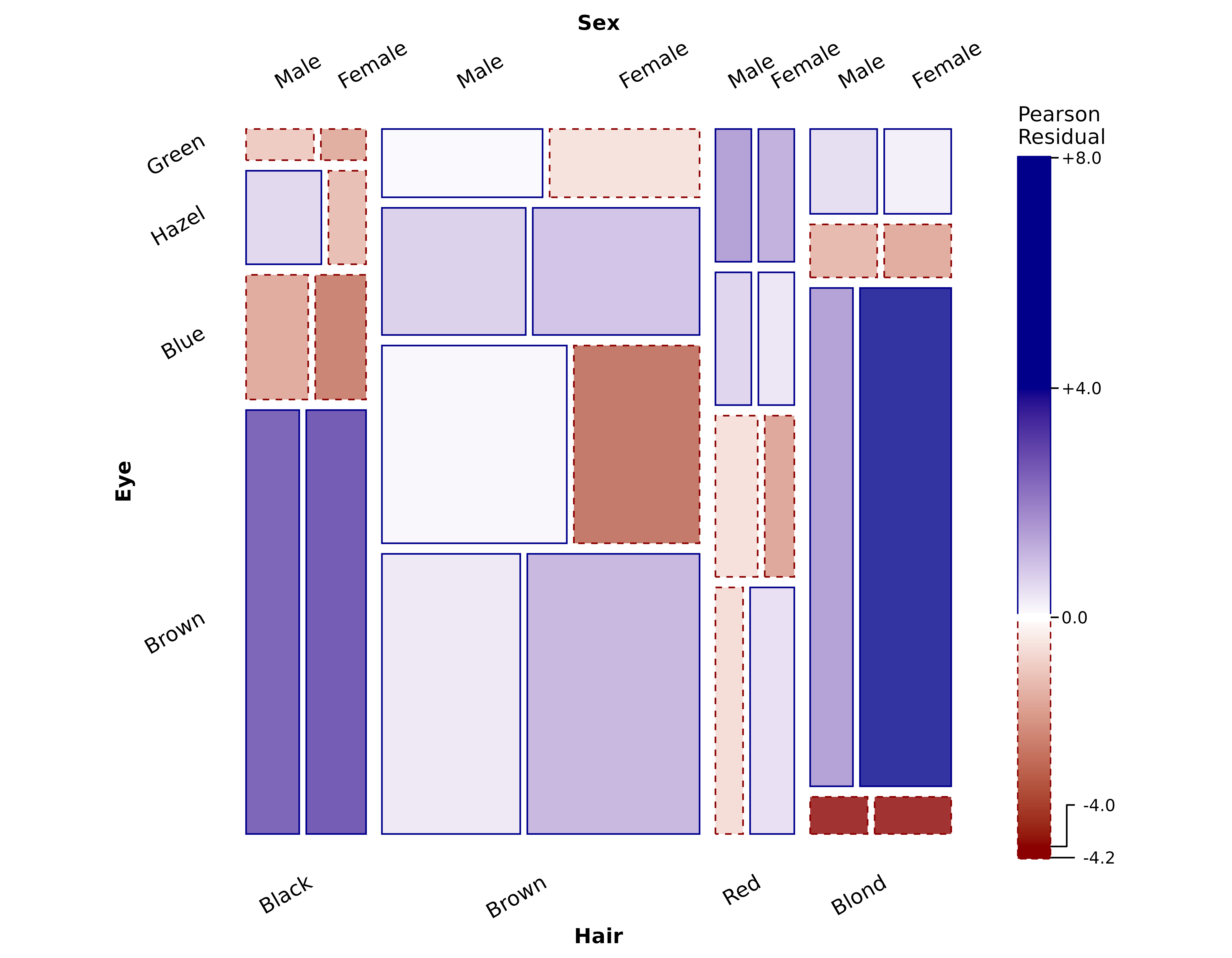

The legend can be re-positioned or disabled through the usual means:

HairEyeColor |>
  as.data.frame() |>
  ggplot(aes(x = product(Sex, Eye, Hair), weight = Freq)) +
  geom_mosaic(expected = "independence") + # `show.legend = FALSE` works as well
  scale_fill_residual(limits = c(-4,4)) +
  theme_mosaic(rot_labels = 30, legend.position = "none")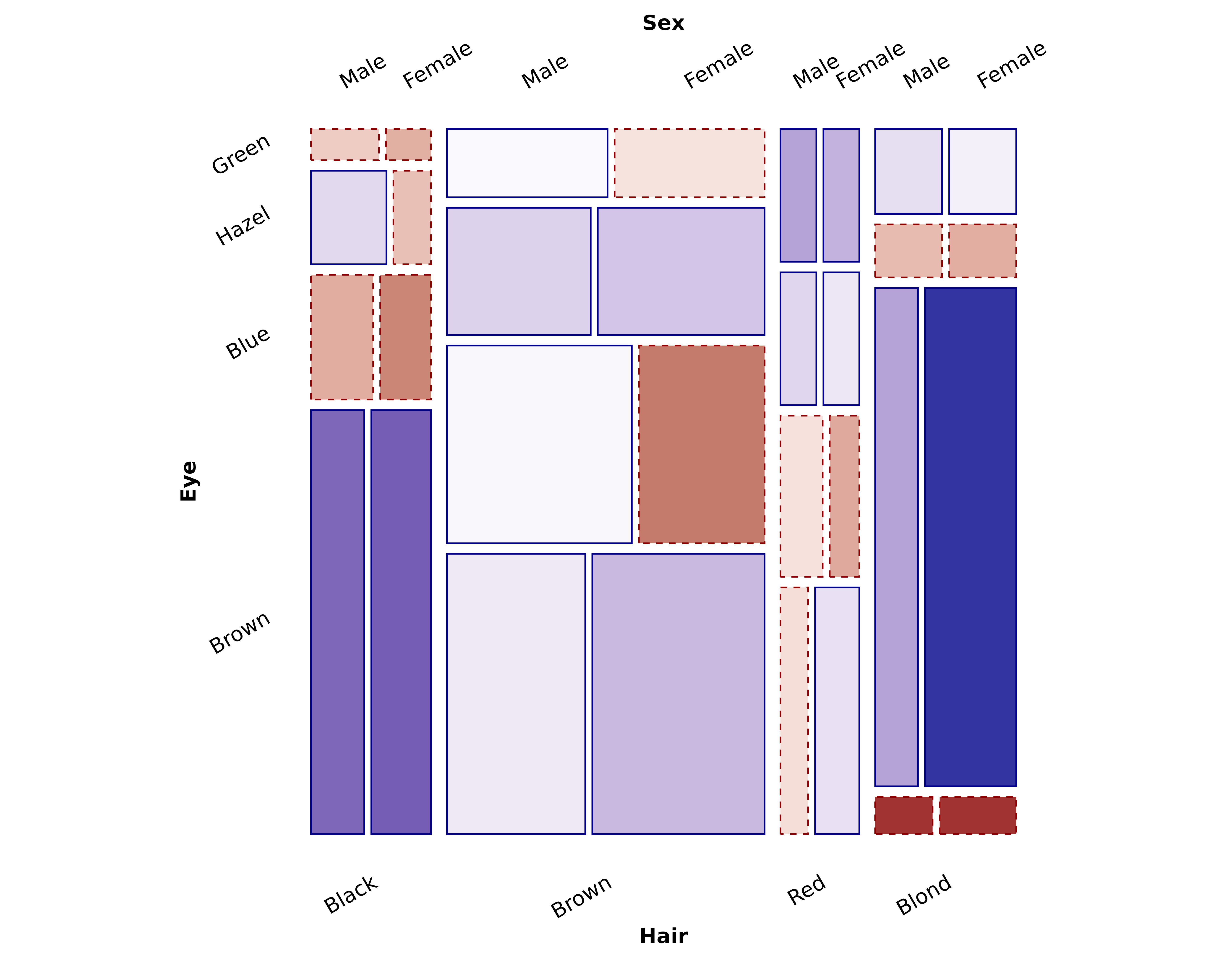

HairEyeColor |>
  as.data.frame() |>
  ggplot(aes(x = product(Sex, Eye, Hair), weight = Freq)) +
  geom_mosaic(expected = "independence") +
  scale_fill_residual(limits = c(-4,4)) +
  theme_mosaic(rot_labels = 30, legend.position = "bottom")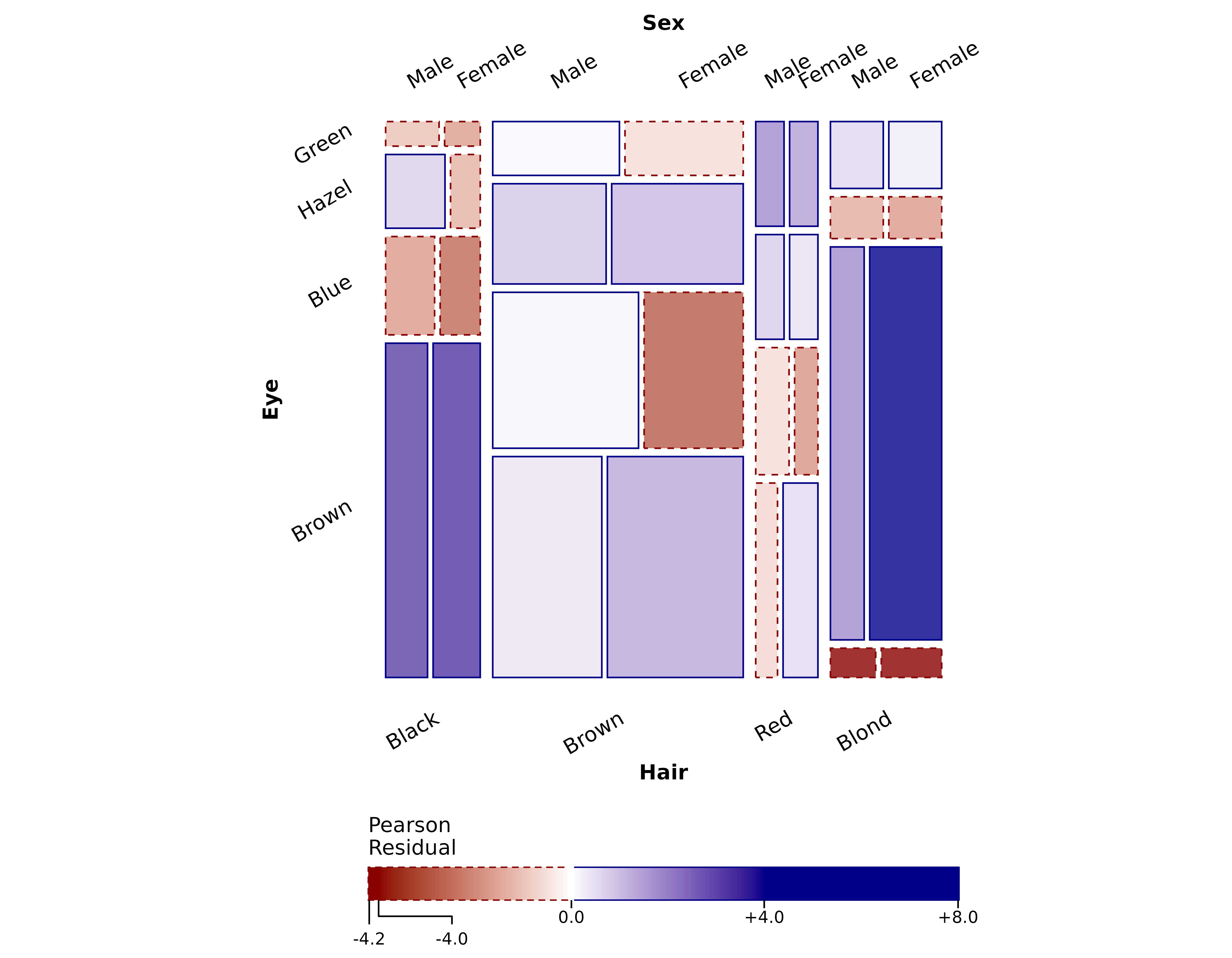

Custom outlines can also be disabled through the usual means:

HairEyeColor |>
  as.data.frame() |>
  ggplot(aes(x = product(Sex, Eye, Hair), weight = Freq)) +
  geom_mosaic(expected = "independence",
              color = NA) +
  scale_fill_residual(limits = c(-4,4)) +
  theme_mosaic(rot_labels = 30, legend.position = "bottom")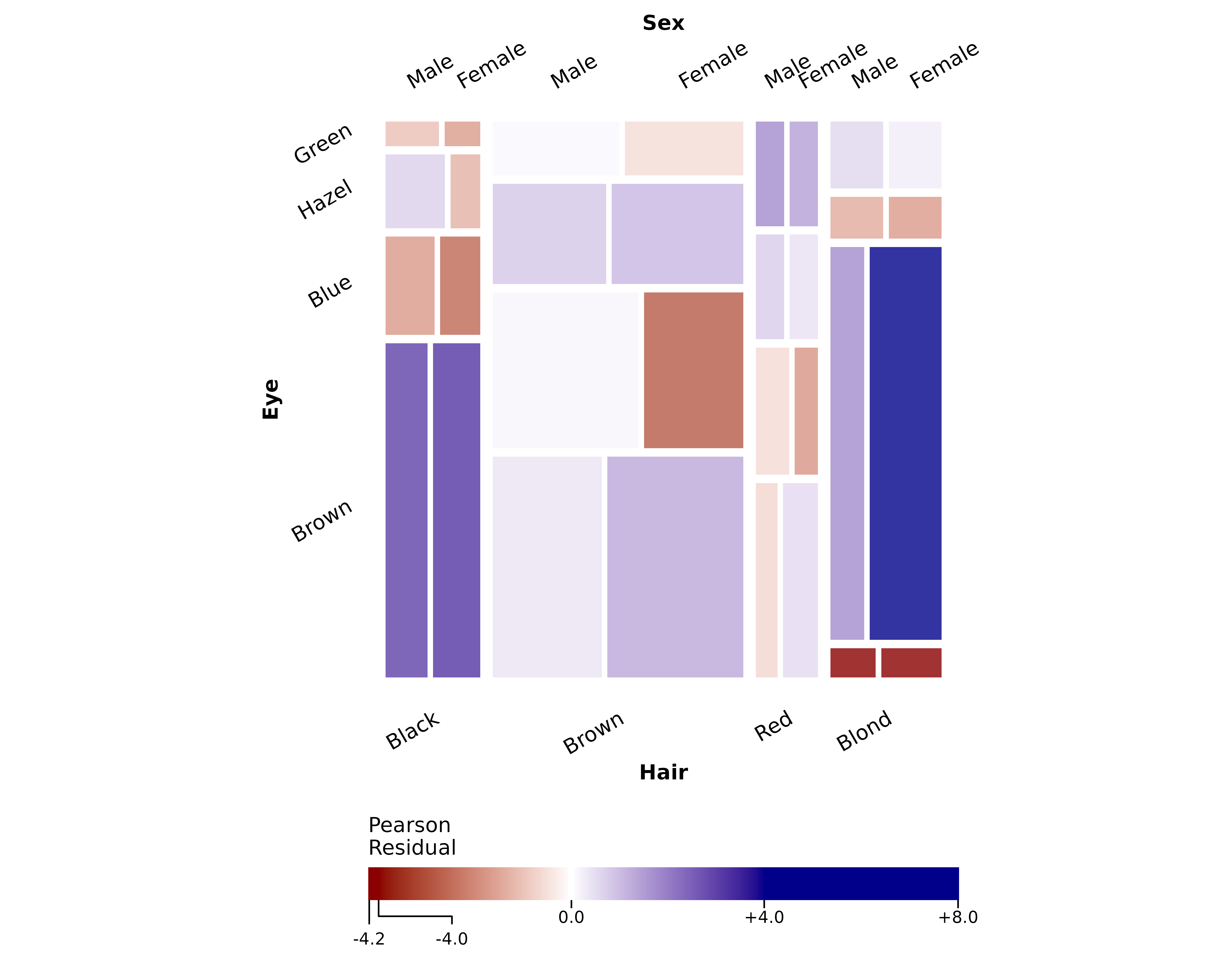

Sharing settings between mosaic layers

When a plot contains multiple mosaic layers (e.g., geom_mosaic() and geom_mosaic_text()), mosaic_settings() can be used to set the divider, offset, and expected arguments once and share them across compatible layers.

In this example, rather than repeating expected = "independence" in each mosaic layer, we specify it once using mosaic_settings():

HairEyeColor |>
  as.data.frame() |>
  ggplot(aes(x = product(Sex, Eye, Hair), weight = Freq)) +
  mosaic_settings(expected = "independence") +
  geom_mosaic() +
  geom_mosaic_text(display_values = "residual",
                   format_digits = 1) +
  scale_fill_residual(limits = c(-4,4)) +
  theme_mosaic(rot_labels = 30)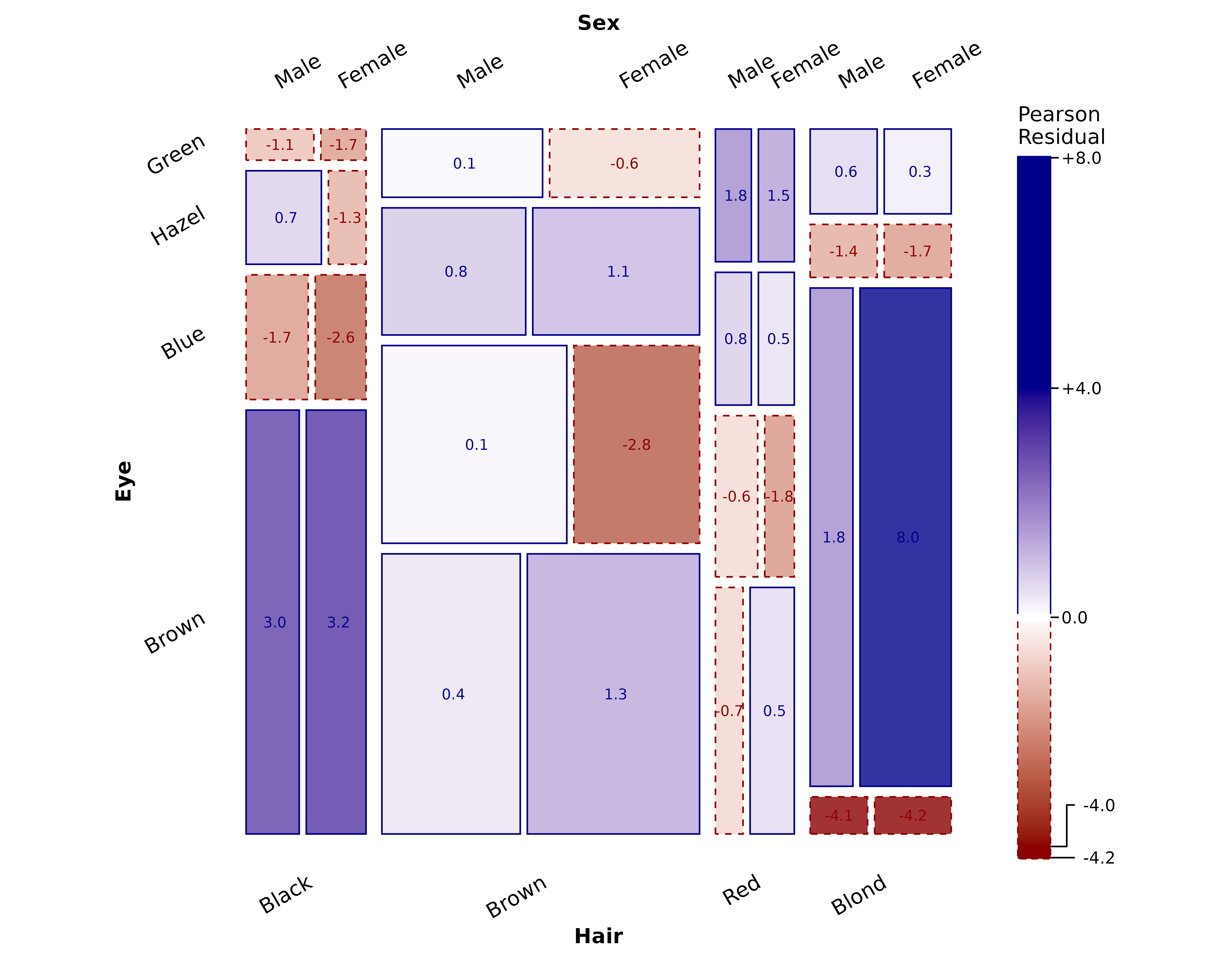

Other fixes/changes

• Fixed namespace-only usage (issue #82 from haleyjeppson/ggmosaic)
• Allow theme_mosaic() to take additional ggplot2::theme() arguments through ...
• Allow for variables created within geom_mosaic() aesthetics (issue #59 from haleyjeppson/ggmosaic)
  • This change also fixed item (re)ordering (issue #77 from haleyjeppson/ggmosaic)
• Fixed fill aesthetic automatically appearing in labels (issue #39 from haleyjeppson/ggmosaic)

References

Friendly, M. (1994). Mosaic displays for multi-way contingency tables. Journal of the American Statistical Association, 89, 190–200.