Chi Square Quantile-Quantile plots

A chi square quantile-quantile plots show the relationship between data-based values which should be distributed as $\chi^2$ and corresponding quantiles from the $\chi^2$ distribution. In multivariate analyses, this is often used both to assess multivariate normality and check for or identify outliers.

For a data frame of numeric variables or a matrix supplied as the argument x, it uses the Mahalanobis squared distances ($D^2$) of observations $\mathbf{x}$ from the centroid $\bar{\mathbf{x}}$ taking the sample covariance matrix $\mathbf{S}$ into account, $$ D^2 = (\mathbf{x} - \bar{\mathbf{x}})^\prime \; \mathbf{S}^{-1} \; (\mathbf{x} - \bar{\mathbf{x}}) \; . $$

The method for "mlm" objects fit using lm for a multivariate response applies this to the residuals from the model.

Usage

cqplot(x, ...)

# S3 method for class 'mlm'
cqplot(x, ...)

# Default S3 method
cqplot(
  x,
  method = c("classical", "mcd", "mve"),
  detrend = FALSE,
  pch = 19,
  col = palette()[1],
  cex = par("cex"),
  ref.col = "red",
  ref.lwd = 2,
  conf = 0.95,
  env.col = "gray",
  env.lwd = 2,
  env.lty = 1,
  env.fill = TRUE,
  fill.alpha = 0.2,
  fill.color = trans.colors(ref.col, fill.alpha),
  labels = if (!is.null(rownames(x))) rownames(x) else 1:nrow(x),
  id.n,
  id.method = "r",
  id.cex = 1,
  id.col = palette()[1],
  xlab,
  ylab,
  main,
  what = deparse(substitute(x)),
  ylim,
  ...
)

Arguments

x: either a numeric data frame or matrix for the default method, or an object of class "mlm" representing a multivariate linear model. In the latter case, residuals from the model are plotted.
...: Other arguments passed to methods
method: estimation method used for center and covariance, one of: "classical" (product-moment), "mcd" (minimum covariance determinant), or "mve" (minimum volume ellipsoid).
detrend: logical; if FALSE, the plot shows values of $D^2$ vs. $\chi^2$. if TRUE, the ordinate shows values of $D^2 - \chi^2$
pch: plot symbol for points. Can be a vector of length equal to the number of rows in x.
col: color for points. Can be a vector of length equal to the number of rows in x. The default is the first entry in the current color palette (see palette and par).
cex: character symbol size for points. Can be a vector of length equal to the number of rows in x.
ref.col: Color for the reference line
ref.lwd: Line width for the reference line
conf: confidence coverage for the approximate confidence envelope
env.col: line color for the boundary of the confidence envelope
env.lwd: line width for the confidence envelope
env.lty: line type for the confidence envelope
env.fill: logical; should the confidence envelope be filled?
fill.alpha: transparency value for fill.color
fill.color: color used to fill the confidence envelope
labels: vector of text strings to be used to identify points, defaults to rownames(x) or observation numbers if rownames(x) is NULL
id.n: number of points labeled. If id.n=0, the default, no point identification occurs.
id.method: point identification method. The default id.method="r" will identify the id.n points with the largest value of abs(y), i.e., the largest Mahalanobis DSQ. See showLabels for other options.
id.cex: size of text for point labels
id.col: color for point labels
xlab: label for horizontal (theoretical quantiles) axis
ylab: label for vertical (empirical quantiles) axis
main: plot title
what: the name of the object plotted; used in the construction of main when that is not specified.
ylim: limits for vertical axis. If not specified, the range of the confidence envelope is used.

Value

Returns invisibly a data.frame containing squared Mahalanobis distances (DSQ), their quantiles and p-values corresponding to the rows of x or the residuals of the model for the identified points, else NULL if no points are identified.

Details

cqplot is a more general version of similar functions in other packages that produce chi square QQ plots. It allows for classical Mahalanobis squared distances as well as robust estimates based on the MVE and MCD; it provides an approximate confidence (concentration) envelope around the line of unit slope, a detrended version, where the reference line is horizontal, the ability to identify or label unusual points, and other graphical features.

Cases with any missing values are excluded from the calculation and graph with a warning.

Confidence envelope

In the typical use of QQ plots, it essential to have something in the nature of a confidence band around the points to be able to appreciate whether, and to what degree the observed data points differ from the reference distribution. For cqplot, this helps to assess whether the data are reasonably distributed as multivariate normal and also to flag potential outliers.

The calculation of the confidence envelope here follows that used in the SAS program, http://www.datavis.ca/sasmac/cqplot.html which comes from Chambers et al. (1983), Section 6.8.

The essential formula computes the standard errors as: $$ \text{se} ( D^2_{(i)} ) = \frac{\hat{b}} {d ( q_i)} \times \sqrt{ p_i (1-p_i) / n } $$ where $D^2_{(i)}$ is the i-th ordered value of $D^2$, $\hat{b}$ is an estimate of the slope of the reference line obtained from the ratio of the interquartile range of the $D^2$ values to that of the $\chi^2_p$ distribution and $d(q_i)$ is the density of the chi square distribution at the quantile $q_i$.

The pointwise confidence envelope of coverage conf = $1-\alpha$ is then calculated as $D^2_{(i)} \pm z_{1-\alpha/2} \text{se} ( D^2_{(i)} )$

Note that this confidence envelope applies only to the $D^2$ computed using the classical estimates of location ($\bar{\mathbf{x}}$) and scatter ($\mathbf{S}$). The qqPlot function provides for simulated envelopes, but only for a univariate measure. Oldford (2016) provides a general theory and methods for QQ plots.

References

J. Chambers, W. S. Cleveland, B. Kleiner, P. A. Tukey (1983). Graphical methods for data analysis, Wadsworth.

R. W. Oldford (2016), "Self calibrating quantile-quantile plots", The American Statistician, 70, 74-90.

Author

Michael Friendly

Examples



cqplot(iris[, 1:4])


iris.mod <- lm(as.matrix(iris[,1:4]) ~ Species, data=iris)
out <- cqplot(iris.mod, id.n=3)

# show return value
out
#>          DSQ quantile           p
#> 119 17.41948 15.77709 0.003333333
#> 135 16.04843 13.27670 0.010000000
#> 42  16.01501 12.09388 0.016666667

# compare with car::qqPlot
car::qqPlot(Mahalanobis(iris[, 1:4]), dist="chisq", df=4)

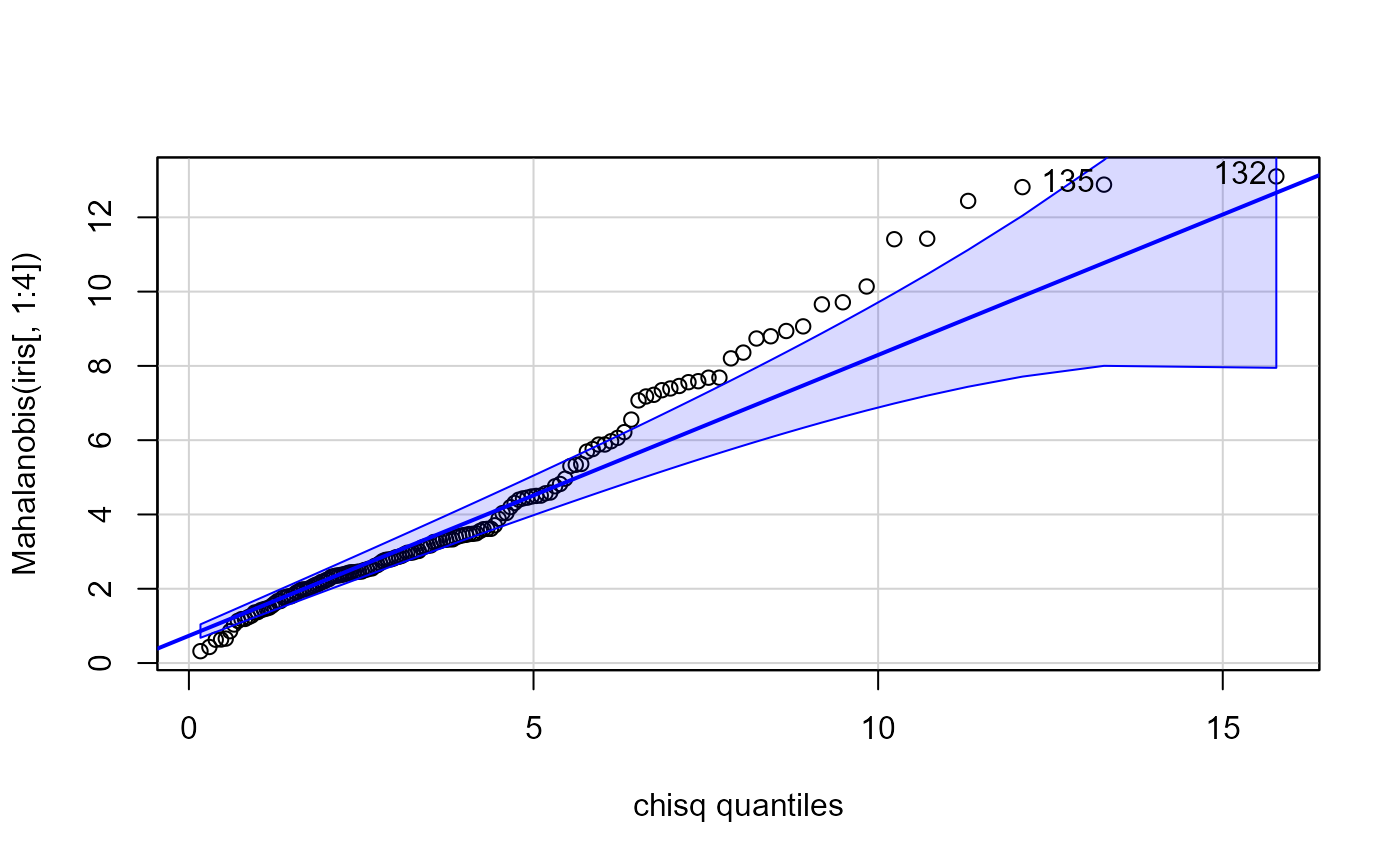#> [1] 132 135


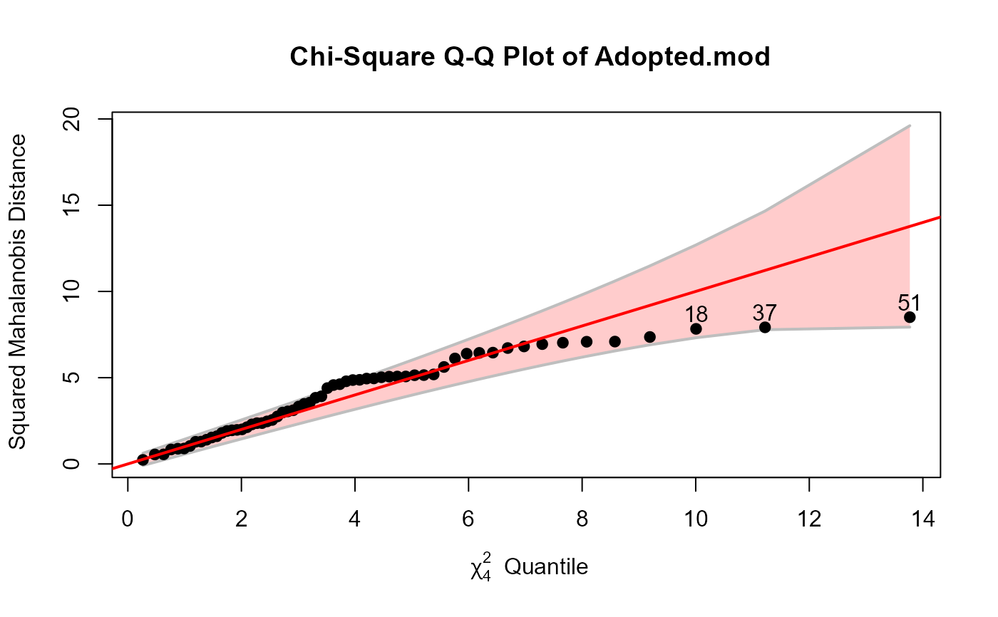
# Adopted data
Adopted.mod <- lm(cbind(Age2IQ, Age4IQ, Age8IQ, Age13IQ) ~ AMED + BMIQ, 
                  data=Adopted)
cqplot(Adopted.mod, id.n=3)

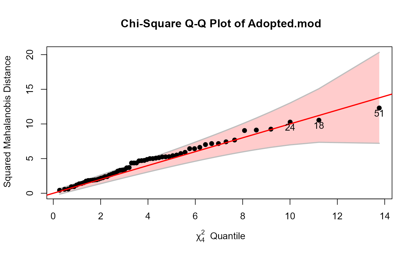
cqplot(Adopted.mod, id.n=3, method="mve")



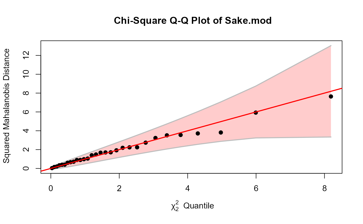
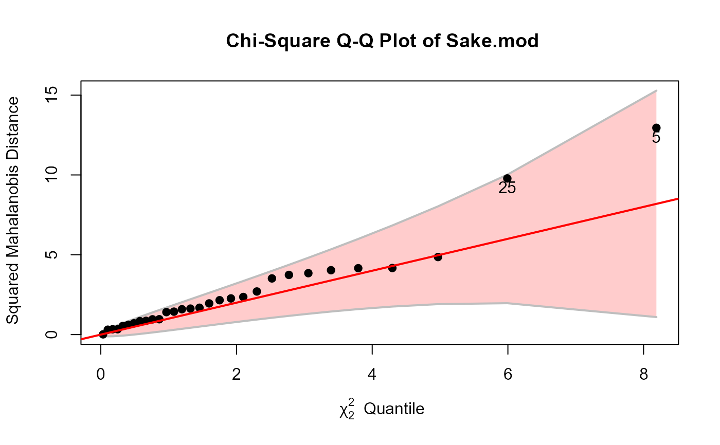
# Sake data
Sake.mod <- lm(cbind(taste, smell) ~ ., data=Sake)
cqplot(Sake.mod)

cqplot(Sake.mod, method="mve", id.n=2)


# SocialCog data -- one extreme outlier
data(SocialCog)
SC.mlm <-  lm(cbind(MgeEmotions,ToM, ExtBias, PersBias) ~ Dx,
               data=SocialCog)
cqplot(SC.mlm, id.n=1)


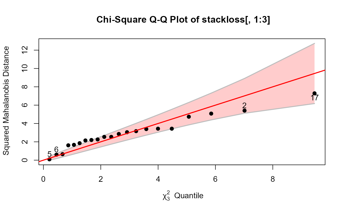
# data frame example: stackloss data
data(stackloss)
cqplot(stackloss[, 1:3], id.n=4)                # very strange

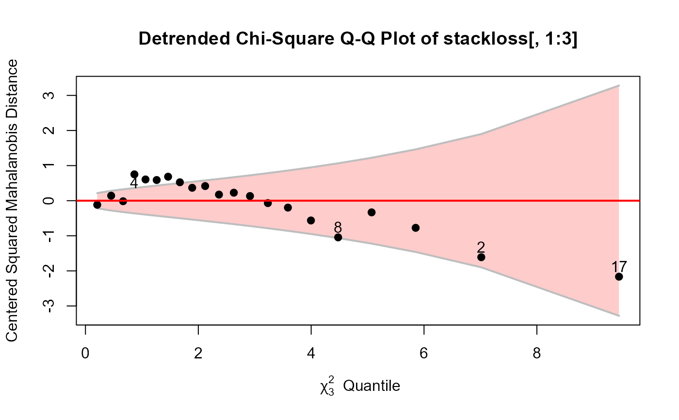
cqplot(stackloss[, 1:3], id.n=4, detrend=TRUE)

cqplot(stackloss[, 1:3], id.n=4, method="mve")

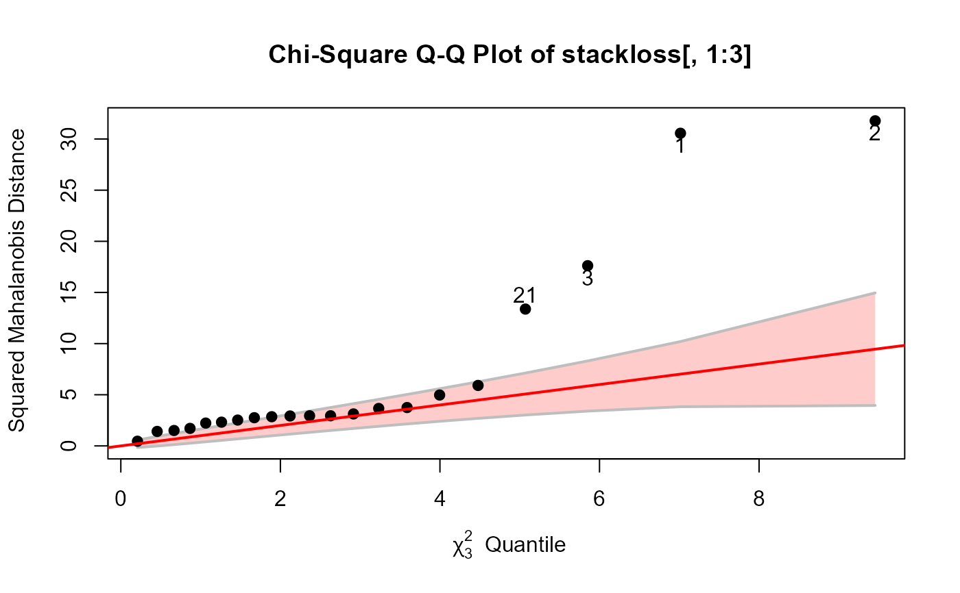cqplot(stackloss[, 1:3], id.n=4, method="mcd")