Regression Deletion Diagnostics for Multivariate Linear Models

This collection of functions is designed to compute regression deletion diagnostics for multivariate linear models following Barrett & Ling (1992) that are close analogs of methods for univariate and generalized linear models handled by the influence.measures in the stats package.

Usage

# S3 method for mlm
influence(model, do.coef = TRUE, m = 1, ...)

Arguments

model: An mlm object, as returned by lm
do.coef: logical. Should the coefficients be returned in the inflmlm object?
m: Size of the subsets for deletion diagnostics
...: Other arguments passed to methods

Value

influence.mlm returns an S3 object of class inflmlm, a list with the following components

m: Deletion subset size
H: Hat values, \(H_I\). If m=1, a vector of diagonal entries of the ‘hat’ matrix. Otherwise, a list of \(m \times m\) matrices corresponding to the subsets.
Q: Residuals, \(Q_I\).
CookD: Cook's distance values
L: Leverage components
R: Residual components
subsets: Indices of the observations in the subsets of size m
labels: Observation labels
call: Model call for the mlm object
Beta: Deletion regression coefficients-- included ifdo.coef=TRUE

Details

In addition, the functions provide diagnostics for deletion of subsets of observations of size m>1.

influence.mlm is a simple wrapper for the computational function, mlm.influence designed to provide an S3 method for class "mlm" objects.

There are still infelicities in the methods for the m>1 case in the current implementation. In particular, for m>1, you must call influence.mlm directly, rather than using the S3 generic influence().

References

Barrett, B. E. and Ling, R. F. (1992). General Classes of Influence Measures for Multivariate Regression. Journal of the American Statistical Association, 87(417), 184-191.

Author

Michael Friendly

Examples


# Rohwer data
data(Rohwer, package="heplots")
Rohwer2 <- subset(Rohwer, subset=group==2)
rownames(Rohwer2)<- 1:nrow(Rohwer2)
Rohwer.mod <- lm(cbind(SAT, PPVT, Raven) ~ n+s+ns+na+ss, data=Rohwer2)

# m=1 diagnostics
influence(Rohwer.mod) |> head()
#> $m
#> [1] 1
#> 
#> $H
#>  [1] 0.1670 0.2185 0.1417 0.0731 0.5682 0.1543 0.0453 0.1766 0.0513 0.4516
#> [11] 0.1454 0.1705 0.1037 0.1265 0.3325 0.3318 0.1732 0.2635 0.2984 0.0788
#> [21] 0.1402 0.1938 0.0446 0.2064 0.1571 0.1533 0.3673 0.1119 0.3043 0.0866
#> [31] 0.0892 0.0732
#> 
#> $Q
#>  [1] 0.1529 0.0378 0.1207 0.0204 0.3439 0.0218 0.1288 0.1930 0.1817 0.0324
#> [11] 0.0725 0.1574 0.0949 0.2997 0.0105 0.0823 0.1925 0.0497 0.1340 0.1093
#> [21] 0.2495 0.0479 0.1572 0.0815 0.3820 0.0641 0.2128 0.0706 0.2295 0.1201
#> [31] 0.2524 0.1735
#> 
#> $CookD
#>  [1] 0.11067 0.03576 0.07411 0.00645 0.84672 0.01458 0.02530 0.14768 0.04040
#> [10] 0.06339 0.04568 0.11629 0.04267 0.16427 0.01519 0.11832 0.14448 0.05671
#> [19] 0.17321 0.03733 0.15164 0.04025 0.03036 0.07294 0.26008 0.04261 0.33866
#> [28] 0.03422 0.30260 0.04505 0.09758 0.05503
#> 
#> $L
#>  [1] 0.2005 0.2795 0.1651 0.0789 1.3160 0.1825 0.0475 0.2145 0.0541 0.8235
#> [11] 0.1702 0.2056 0.1158 0.1448 0.4981 0.4966 0.2095 0.3578 0.4252 0.0855
#> [21] 0.1631 0.2404 0.0466 0.2601 0.1864 0.1811 0.5804 0.1260 0.4373 0.0948
#> [31] 0.0980 0.0790
#> 
#> $R
#>  [1] 0.1836 0.0483 0.1406 0.0220 0.7964 0.0258 0.1349 0.2344 0.1915 0.0591
#> [11] 0.0848 0.1898 0.1059 0.3431 0.0158 0.1232 0.2328 0.0674 0.1909 0.1187
#> [21] 0.2902 0.0594 0.1646 0.1028 0.4532 0.0757 0.3363 0.0795 0.3299 0.1315
#> [31] 0.2771 0.1872
#> 

# try an m=2 case
## res2 <- influence.mlm(Rohwer.mod, m=2, do.coef=FALSE)
## res2.df <- as.data.frame(res2)
## head(res2.df)
## scatterplotMatrix(log(res2.df))


influencePlot(Rohwer.mod, id.n=4, type="cookd")

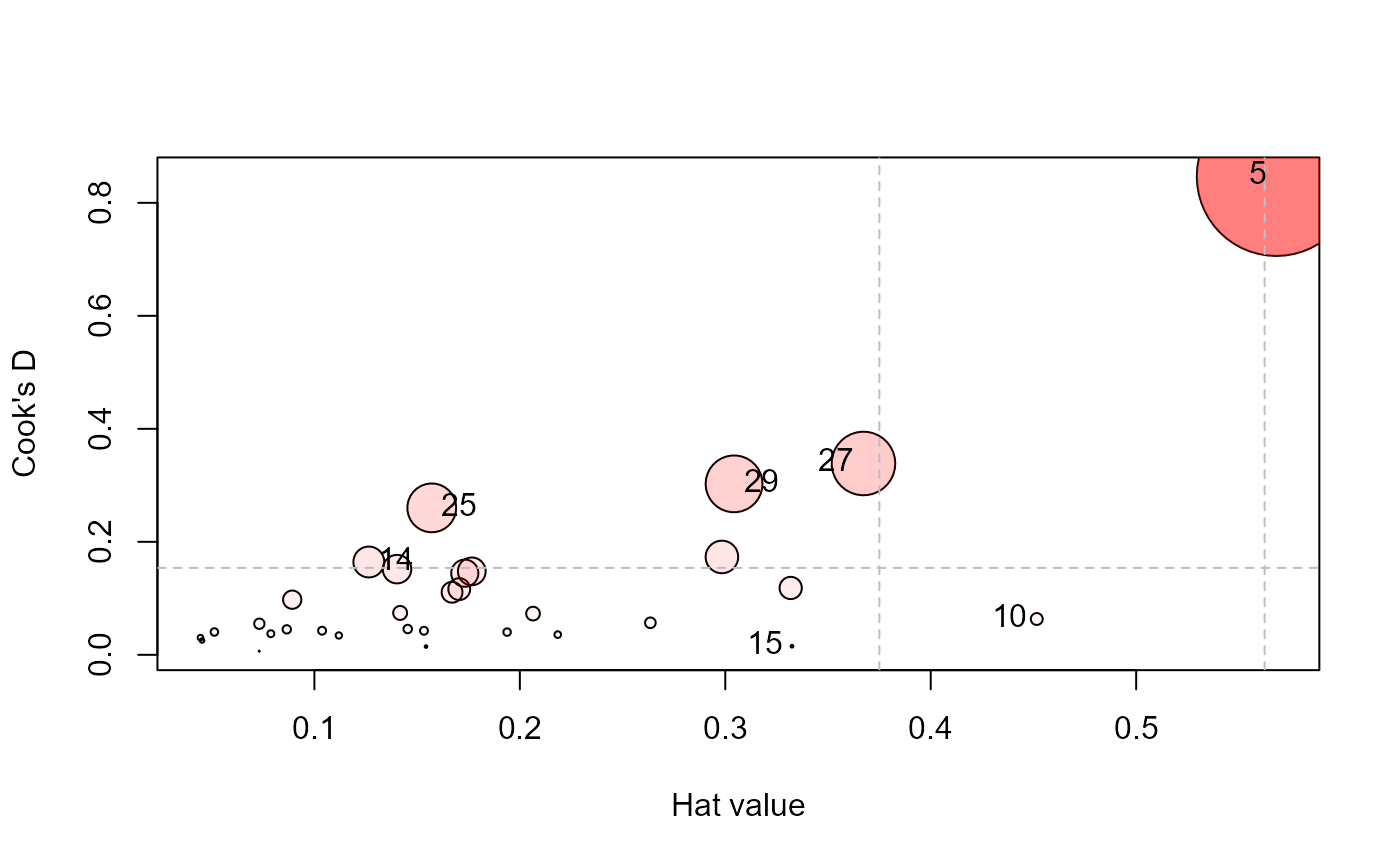#>        H      Q  CookD     L      R
#> 5  0.568 0.3439 0.8467 1.316 0.7964
#> 10 0.452 0.0324 0.0634 0.824 0.0591
#> 14 0.126 0.2997 0.1643 0.145 0.3431
#> 15 0.332 0.0105 0.0152 0.498 0.0158
#> 25 0.157 0.3820 0.2601 0.186 0.4532
#> 27 0.367 0.2128 0.3387 0.580 0.3363
#> 29 0.304 0.2295 0.3026 0.437 0.3299


# Sake data
data(Sake, package="heplots")
Sake.mod <- lm(cbind(taste,smell) ~ ., data=Sake)
influence(Sake.mod)
#> Multivariate influence statistics for model:
#>  lm(formula = cbind(taste, smell) ~ ., data = Sake) 
#>  m= 1 case deletion diagnostics 
#>         H      Q   CookD      L      R
#> 1  0.8116 0.5757 1.09033 4.3086 3.0564
#> 2  0.2975 0.0500 0.03472 0.4234 0.0712
#> 3  0.0897 0.0711 0.01490 0.0986 0.0782
#> 4  0.1581 0.1729 0.06379 0.1878 0.2054
#> 5  0.1954 0.4069 0.18550 0.2428 0.5057
#> 6  0.2772 0.0255 0.01652 0.3835 0.0353
#> 7  0.2294 0.2042 0.10928 0.2977 0.2649
#> 8  0.3536 0.0546 0.04506 0.5471 0.0845
#> 9  0.2128 0.2124 0.10548 0.2704 0.2698
#> 10 0.2559 0.0923 0.05510 0.3439 0.1240
#> 11 0.2768 0.2131 0.13763 0.3827 0.2947
#> 12 0.1756 0.0848 0.03474 0.2129 0.1029
#> 13 0.0926 0.1556 0.03364 0.1021 0.1715
#> 14 0.2033 0.0485 0.02301 0.2551 0.0609
#> 15 0.4379 0.0168 0.01717 0.7789 0.0299
#> 16 0.0932 0.0917 0.01995 0.1028 0.1012
#> 17 0.2638 0.0668 0.04109 0.3583 0.0907
#> 18 0.1969 0.0213 0.00978 0.2451 0.0265
#> 19 0.3102 0.0150 0.01088 0.4497 0.0218
#> 20 0.1747 0.1386 0.05651 0.2117 0.1679
#> 21 0.6017 0.2129 0.29893 1.5107 0.5346
#> 22 0.4220 0.1444 0.14223 0.7302 0.2499
#> 23 0.4737 0.1119 0.12364 0.9001 0.2125
#> 24 0.3005 0.1197 0.08395 0.4297 0.1712
#> 25 0.3250 0.4486 0.34018 0.4815 0.6646
#> 26 0.2875 0.1307 0.08767 0.4035 0.1834
#> 27 0.1421 0.0157 0.00519 0.1657 0.0182
#> 28 0.7408 0.0167 0.02889 2.8583 0.0645
#> 29 0.3058 0.1606 0.11458 0.4406 0.2313
#> 30 0.2946 0.1552 0.10670 0.4177 0.2200
influencePlot(Sake.mod, id.n=3, type="cookd")

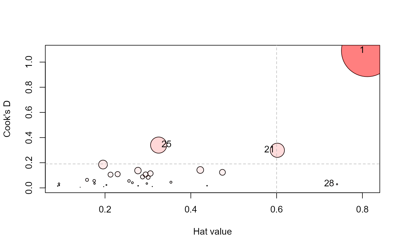#>        H      Q  CookD     L      R
#> 1  0.812 0.5757 1.0903 4.309 3.0564
#> 21 0.602 0.2129 0.2989 1.511 0.5346
#> 25 0.325 0.4486 0.3402 0.481 0.6646
#> 28 0.741 0.0167 0.0289 2.858 0.0645