Regression LR Influence Plot

This function creates a “bubble” plot of functions, R = log(Studentized residuals^2) by L = log(H/p*(1-H)) of the hat values, with the areas of the circles representing the observations proportional to Cook's distances.

Usage

lrPlot(model, ...)

# S3 method for lm
lrPlot(
  model,
  scale = 12,
  xlab = "log Leverage factor [log H/p*(1-H)]",
  ylab = "log (Studentized Residual^2)",
  xlim = NULL,
  ylim,
  labels,
  id.method = "noteworthy",
  id.n = if (id.method[1] == "identify") Inf else 0,
  id.cex = 1,
  id.col = palette()[1],
  ref = c("h", "v", "d", "c"),
  ref.col = "gray",
  ref.lty = 2,
  ref.lab = TRUE,
  ...
)

Arguments

model: a model object fit by lm
...: arguments to pass to the plot and points functions.
scale: a factor to adjust the radii of the circles, in relation to sqrt(CookD)
xlab, ylab: axis labels.
xlim, ylim: Limits for x and y axes. In the space of (L, R) very small residuals typically extend the y axis enough to swamp the large residuals, so the default for ylim is set to a range of 6 log units starting at the maximum value.
labels, id.method, id.n, id.cex, id.col: settings for labeling points; see link{showLabels} for details. To omit point labeling, set id.n=0, the default. The default id.method="noteworthy" is used in this function to indicate setting labels for points with large Studentized residuals, hat-values or Cook's distances. See Details below. Set id.method="identify" for interactive point identification.
ref: Options to draw reference lines, any one or more of c("h", "v", "d", "c"). "h" and "v" draw horizontal and vertical reference lines at noteworthy values of R and L respectively. "d" draws equally spaced diagonal reference lines for contours of equal CookD. "c" draws diagonal reference lines corresponding to approximate 0.95 and 0.99 contours of CookD.
ref.col, ref.lty: Color and line type for reference lines. Reference lines for "c" %in% ref are handled separately.
ref.lab: A logical, indicating whether the reference lines should be labeled.

Value

If points are identified, returns a data frame with the hat values, Studentized residuals and Cook's distance of the identified points. If no points are identified, nothing is returned. This function is primarily used for its side-effect of drawing a plot.

Details

This plot, suggested by McCulloch & Meeter (1983) has the attractive property that contours of equal Cook's distance are diagonal lines with slope = -1. Various reference lines are drawn on the plot corresponding to twice and three times the average hat value, a “large” squared studentized residual and contours of Cook's distance.

The id.method="noteworthy" setting also requires setting id.n>0 to have any effect. Using id.method="noteworthy", and id.n>0, the number of points labeled is the union of the largest id.n values on each of L, R, and CookD.

References

A. J. Lawrence (1995). Deletion Influence and Masking in Regression Journal of the Royal Statistical Society. Series B (Methodological) , Vol. 57, No. 1, pp. 181-189.

McCulloch, C. E. & Meeter, D. (1983). Discussion of "Outliers..." by R. J. Beckman and R. D. Cook. Technometrics, 25, 152-155.

Author

Michael Friendly

Examples


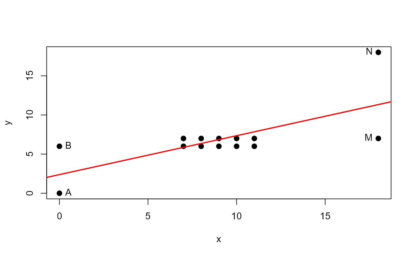
# artificial example from Lawrence (1995)
x <- c( 0, 0, 7, 7, 8, 8, 9, 9, 10, 10, 11, 11, 18, 18 )
y <- c( 0, 6, 6, 7, 6, 7, 6, 7, 6,  7,  6,  7,  7,  18 )
DF <- data.frame(x,y, row.names=LETTERS[1:length(x)])
DF
#>    x  y
#> A  0  0
#> B  0  6
#> C  7  6
#> D  7  7
#> E  8  6
#> F  8  7
#> G  9  6
#> H  9  7
#> I 10  6
#> J 10  7
#> K 11  6
#> L 11  7
#> M 18  7
#> N 18 18

with(DF, {
  plot(x,y, pch=16, cex=1.3)
  abline(lm(y~x), col="red", lwd=2)
  NB <- c(1,2,13,14)
  text(x[NB],y[NB], LETTERS[NB], pos=c(4,4,2,2))
  }
)


mod <- lm(y~x, data=DF)
# standard influence plot from car
influencePlot(mod, id.n=4)
#> Warning: "id.n" is not a graphical parameter
#> Warning: "id.n" is not a graphical parameter
#> Warning: "id.n" is not a graphical parameter
#> Warning: "id.n" is not a graphical parameter
#> Warning: "id.n" is not a graphical parameter
#> Warning: "id.n" is not a graphical parameter
#> Warning: "id.n" is not a graphical parameter

#>   StudRes   Hat CookD
#> M   -2.16 0.307 0.793
#> N    5.16 0.307 1.879

# lrPlot version
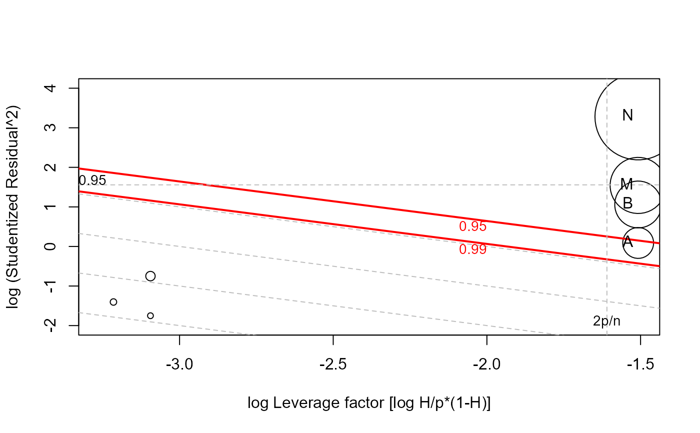
lrPlot(mod, id.n=4)

#> Note: 7 points less than R= -2 have been clipped to preserve resolution
#>   Rstudent   Hat CookD     L      R
#> A    -1.05 0.307 0.240 -1.51 0.0884
#> B     1.70 0.307 0.553 -1.51 1.0612
#> M    -2.16 0.307 0.793 -1.51 1.5427
#> N     5.16 0.307 1.879 -1.51 3.2807


library(car)
dmod <- lm(prestige ~ income + education, data = Duncan)
influencePlot(dmod, id.n=3)
#> Warning: "id.n" is not a graphical parameter
#> Warning: "id.n" is not a graphical parameter
#> Warning: "id.n" is not a graphical parameter
#> Warning: "id.n" is not a graphical parameter
#> Warning: "id.n" is not a graphical parameter
#> Warning: "id.n" is not a graphical parameter
#> Warning: "id.n" is not a graphical parameter

#>             StudRes    Hat CookD
#> minister      3.135 0.1731 0.566
#> reporter     -2.397 0.0544 0.099
#> conductor    -1.704 0.1945 0.224
#> RR.engineer   0.809 0.2691 0.081
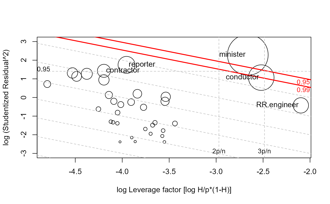
lrPlot(dmod, id.n=3)

#> Note: 11 points less than R= -3 have been clipped to preserve resolution
#>             Rstudent    Hat  CookD     L      R
#> minister       3.135 0.1731 0.5664 -2.66  2.285
#> reporter      -2.397 0.0544 0.0990 -3.95  1.748
#> conductor     -1.704 0.1945 0.2236 -2.52  1.066
#> contractor     2.044 0.0433 0.0585 -4.20  1.430
#> RR.engineer    0.809 0.2691 0.0810 -2.10 -0.424