Computes effects (in the sense of the effects package—see, in
particular, Effect)—for "nestedLogit" models, which then
can be used with other functions in the effects package, for example,
predictorEffects and to produce effect plots.
Usage
# S3 method for class 'nestedLogit'
Effect(
  focal.predictors,
  mod,
  confidence.level = 0.95,
  fixed.predictors = NULL,
  ...
)
Arguments
- focal.predictors
a character vector of the names of one or more of the predictors in the model, for which the effect display should be computed.
- mod
a
"nestedLogit"model object.- confidence.level
for point-wise confidence bands around the effects (the default is
0.95).- fixed.predictors
controls the values at which other predictors are fixed; see
Effectfor details; ifNULL(the default), numeric predictors are set to their means, factors to their distribution in the data.- ...
optional arguments to be passed to the
Effectmethod for binary logit models (fit by theglmfunction).
Value
an object of class "effpoly" (see Effect).
References
John Fox and Sanford Weisberg (2019). An R Companion to Applied Regression, 3rd Edition. Sage, Thousand Oaks, CA.
John Fox, Sanford Weisberg (2018). Visualizing Fit and Lack of Fit in Complex Regression Models with Predictor Effect Plots and Partial Residuals. Journal of Statistical Software, 87(9), 1-27.
Examples
data("Womenlf", package = "carData")
comparisons <- logits(work=dichotomy("not.work",
working=c("parttime", "fulltime")),
full=dichotomy("parttime", "fulltime"))
m <- nestedLogit(partic ~ hincome + children,
dichotomies = comparisons,
data=Womenlf)
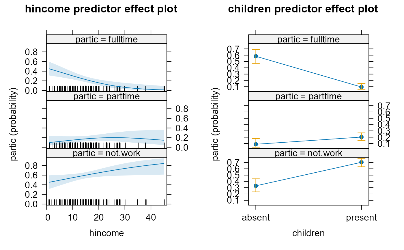
peff.women <- effects::predictorEffects(m)
plot(peff.women)
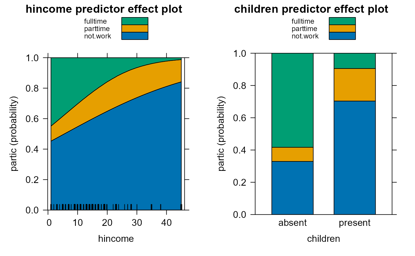
 plot(peff.women, axes=list(y=list(style="stacked")))
 summary(peff.women)
#>
#> hincome predictor effect
#>
#> hincome effect (probability) for not.work
#> hincome
#> 1 1.9 2.8 3.69 4.59 5.49 6.39 7.29
#> 0.4523534 0.4618023 0.4712788 0.4806704 0.4901814 0.4996996 0.5092179 0.5187296
#> 8.18 9.08 9.98 10.9 11.8 12.7 13.6 14.5
#> 0.5281223 0.5376003 0.5470512 0.5566771 0.5660528 0.5753815 0.5846568 0.5938724
#> 15.4 16.3 17.2 18.1 19 19.9 20.8 21.7
#> 0.6030225 0.6121010 0.6211024 0.6300212 0.6388520 0.6475901 0.6562304 0.6647686
#> 22.6 23.4 24.3 25.2 26.1 27 27.9 28.8
#> 0.6732003 0.6806026 0.6888224 0.6969250 0.7049069 0.7127653 0.7204974 0.7281007
#> 29.7 30.6 31.5 32.4 33.3 34.2 35.1 36
#> 0.7355732 0.7429127 0.7501178 0.7571869 0.7641189 0.7709129 0.7775682 0.7840843
#> 36.9 37.8 38.7 39.6 40.5 41.4 42.3 43.2
#> 0.7904609 0.7966981 0.8027959 0.8087547 0.8145751 0.8202576 0.8258033 0.8312131
#> 44.1 45
#> 0.8364881 0.8416297
#>
#> hincome effect (probability) for parttime
#> hincome
#> 1 1.9 2.8 3.69 4.59 5.49 6.39
#> 0.09864534 0.10359265 0.10854405 0.11368937 0.11877884 0.12400783 0.12915775
#> 7.29 8.18 9.08 9.98 10.9 11.8 12.7
#> 0.13440804 0.13956000 0.14473686 0.14972987 0.15465311 0.15983886 0.16389146
#> 13.6 14.5 15.4 16.3 17.2 18.1 19
#> 0.16883681 0.17249633 0.17698253 0.18015718 0.18408391 0.18669457 0.18997787
#> 19.9 20.8 21.7 22.6 23.4 24.3 25.2
#> 0.19289987 0.19453999 0.19673115 0.19769122 0.19970141 0.19998331 0.20067294
#> 26.1 27 27.9 28.8 29.7 30.6 31.5
#> 0.20028308 0.20024010 0.19982683 0.19848381 0.19741243 0.19551731 0.19385571
#> 32.4 33.3 34.2 35.1 36 36.9 37.8
#> 0.19147712 0.18930194 0.18651379 0.18390586 0.18078344 0.17782378 0.17470521
#> 38.7 39.6 40.5 41.4 42.3 43.2 44.1
#> 0.17120718 0.16785358 0.16419793 0.16067852 0.15692500 0.15330158 0.14950269
#> 45
#> 0.14582907
#>
#> hincome effect (probability) for fulltime
#> hincome
#> 1 1.9 2.8 3.69 4.59 5.49 6.39
#> 0.44900129 0.43460502 0.42017715 0.40564022 0.39103972 0.37629259 0.36162433
#> 7.29 8.18 9.08 9.98 10.9 11.8 12.7
#> 0.34686236 0.33231772 0.31766287 0.30321897 0.28866980 0.27410834 0.26072707
#> 13.6 14.5 15.4 16.3 17.2 18.1 19
#> 0.24650643 0.23363123 0.21999498 0.20774179 0.19481368 0.18328427 0.17117008
#> 19.9 20.8 21.7 22.6 23.4 24.3 25.2
#> 0.15951007 0.14922960 0.13850025 0.12910846 0.11969604 0.11119425 0.10240207
#> 26.1 27 27.9 28.8 29.7 30.6 31.5
#> 0.09480998 0.08699458 0.07967577 0.07341545 0.06701441 0.06156996 0.05602651
#> 32.4 33.3 34.2 35.1 36 36.9 37.8
#> 0.05133597 0.04657912 0.04257327 0.03852592 0.03513225 0.03171528 0.02859670
#> 38.7 39.6 40.5 41.4 42.3 43.2 44.1
#> 0.02599692 0.02339170 0.02122701 0.01906384 0.01727168 0.01548533 0.01400918
#> 45
#> 0.01254120
#>
#> Lower 95 Percent Confidence Limits for not.work
#> hincome
#> 1 1.9 2.8 3.69 4.59 5.49 6.39 7.29
#> 0.3159695 0.3310511 0.3463719 0.3617049 0.3773328 0.3930128 0.4086632 0.4241902
#> 8.18 9.08 9.98 10.9 11.8 12.7 13.6 14.5
#> 0.4393183 0.4542674 0.4687299 0.4828570 0.4958777 0.5079597 0.5189802 0.5288600
#> 15.4 16.3 17.2 18.1 19 19.9 20.8 21.7
#> 0.5375785 0.5451759 0.5517427 0.5574002 0.5622799 0.5665088 0.5702001 0.5734503
#> 22.6 23.4 24.3 25.2 26.1 27 27.9 28.8
#> 0.5763392 0.5786565 0.5810295 0.5831958 0.5851899 0.5870396 0.5887674 0.5903915
#> 29.7 30.6 31.5 32.4 33.3 34.2 35.1 36
#> 0.5919270 0.5933862 0.5947793 0.5961148 0.5974000 0.5986407 0.5998422 0.6010089
#> 36.9 37.8 38.7 39.6 40.5 41.4 42.3 43.2
#> 0.6021445 0.6032522 0.6043348 0.6053948 0.6064343 0.6074552 0.6084592 0.6094476
#> 44.1 45
#> 0.6104217 0.6113828
#>
#> Lower 95 Percent Confidence Limits for parttime
#> hincome
#> 1 1.9 2.8 3.69 4.59 5.49 6.39
#> 0.03847131 0.04276604 0.04735083 0.05237580 0.05766875 0.06338466 0.06932277
#> 7.29 8.18 9.08 9.98 10.9 11.8 12.7
#> 0.07562710 0.08206002 0.08872208 0.09531895 0.10190947 0.10865531 0.11405577
#> 13.6 14.5 15.4 16.3 17.2 18.1 19
#> 0.12001554 0.12428948 0.12878012 0.13151369 0.13424863 0.13536112 0.13643431
#> 19.9 20.8 21.7 22.6 23.4 24.3 25.2
#> 0.13676393 0.13586219 0.13501729 0.13317007 0.13208517 0.12954146 0.12715419
#> 26.1 27 27.9 28.8 29.7 30.6 31.5
#> 0.12406951 0.12116163 0.11802865 0.11436509 0.11089064 0.10698659 0.10327582
#> 32.4 33.3 34.2 35.1 36 36.9 37.8
#> 0.09923212 0.09538532 0.09129674 0.08740835 0.08336110 0.07951628 0.07571321
#> 38.7 39.6 40.5 41.4 42.3 43.2 44.1
#> 0.07185586 0.06820070 0.06454437 0.06108654 0.05766792 0.05444130 0.05128269
#> 45
#> 0.04830710
#>
#> Lower 95 Percent Confidence Limits for fulltime
#> hincome
#> 1 1.9 2.8 3.69 4.59 5.49
#> 0.311275740 0.303984689 0.296573453 0.288937743 0.281161091 0.273127893
#> 6.39 7.29 8.18 9.08 9.98 10.9
#> 0.264972521 0.256539050 0.247988764 0.239080389 0.229964345 0.220368072
#> 11.8 12.7 13.6 14.5 15.4 16.3
#> 0.210239105 0.200459222 0.189418729 0.178861142 0.167036383 0.155895357
#> 17.2 18.1 19 19.9 20.8 21.7
#> 0.143650271 0.132406067 0.120351187 0.108642000 0.098350645 0.087704592
#> 22.6 23.4 24.3 25.2 26.1 27
#> 0.078576692 0.069613542 0.061804111 0.053997739 0.047553785 0.041196107
#> 27.9 28.8 29.7 30.6 31.5 32.4
#> 0.035543805 0.030976068 0.026541740 0.022997990 0.019587626 0.016887733
#> 33.3 34.2 35.1 36 36.9 37.8
#> 0.014308889 0.012283444 0.010361274 0.008861644 0.007446381 0.006245988
#> 38.7 39.6 40.5 41.4 42.3 43.2
#> 0.005317145 0.004446673 0.003775970 0.003149807 0.002669044 0.002221675
#> 44.1 45
#> 0.001879189 0.001561390
#>
#> Upper 95 Percent Confidence Limits for not.work
#> hincome
#> 1 1.9 2.8 3.69 4.59 5.49 6.39 7.29
#> 0.5962883 0.5980285 0.5998890 0.6018689 0.6040398 0.6064137 0.6090323 0.6119467
#> 8.18 9.08 9.98 10.9 11.8 12.7 13.6 14.5
#> 0.6151814 0.6188841 0.6231101 0.6280763 0.6336758 0.6401102 0.6474575 0.6557532
#> 15.4 16.3 17.2 18.1 19 19.9 20.8 21.7
#> 0.6649766 0.6750482 0.6858407 0.6971996 0.7089624 0.7209753 0.7331010 0.7452227
#> 22.6 23.4 24.3 25.2 26.1 27 27.9 28.8
#> 0.7572438 0.7677810 0.7794113 0.7907560 0.8017765 0.8124433 0.8227350 0.8326368
#> 29.7 30.6 31.5 32.4 33.3 34.2 35.1 36
#> 0.8421394 0.8512380 0.8599317 0.8682226 0.8761155 0.8836175 0.8907373 0.8974849
#> 36.9 37.8 38.7 39.6 40.5 41.4 42.3 43.2
#> 0.9038717 0.9099097 0.9156116 0.9209906 0.9260599 0.9308333 0.9353240 0.9395456
#> 44.1 45
#> 0.9435113 0.9472341
#>
#> Upper 95 Percent Confidence Limits for parttime
#> hincome
#> 1 1.9 2.8 3.69 4.59 5.49 6.39 7.29
#> 0.2303876 0.2301342 0.2297475 0.2294036 0.2289148 0.2284694 0.2279869 0.2276258
#> 8.18 9.08 9.98 10.9 11.8 12.7 13.6 14.5
#> 0.2273707 0.2272957 0.2273933 0.2277713 0.2289403 0.2298530 0.2322760 0.2343960
#> 15.4 16.3 17.2 18.1 19 19.9 20.8 21.7
#> 0.2382923 0.2417837 0.2471379 0.2518255 0.2582505 0.2650038 0.2706237 0.2776004
#> 22.6 23.4 24.3 25.2 26.1 27 27.9 28.8
#> 0.2832578 0.2903517 0.2957168 0.3019922 0.3069096 0.3125739 0.3178821 0.3219802
#> 29.7 30.6 31.5 32.4 33.3 34.2 35.1 36
#> 0.3266412 0.3302172 0.3342662 0.3373568 0.3408474 0.3434981 0.3464878 0.3487438
#> 36.9 37.8 38.7 39.6 40.5 41.4 42.3 43.2
#> 0.3512872 0.3536093 0.3553357 0.3572844 0.3587123 0.3603271 0.3614863 0.3628022
#> 44.1 45
#> 0.3637196 0.3647681
#>
#> Upper 95 Percent Confidence Limits for fulltime
#> hincome
#> 1 1.9 2.8 3.69 4.59 5.49 6.39
#> 0.59501785 0.57498523 0.55467452 0.53407517 0.51320236 0.49204610 0.47094270
#> 7.29 8.18 9.08 9.98 10.9 11.8 12.7
#> 0.44974914 0.42896528 0.40821763 0.38804929 0.36814483 0.34881095 0.33159955
#> 13.6 14.5 15.4 16.3 17.2 18.1 19
#> 0.31413172 0.29906450 0.28401891 0.27128922 0.25869488 0.24812169 0.23765017
#> 19.9 20.8 21.7 22.6 23.4 24.3 25.2
#> 0.22810055 0.22000694 0.21188244 0.20490995 0.19813645 0.19197757 0.18568011
#> 26.1 27 27.9 28.8 29.7 30.6 31.5
#> 0.18014460 0.17444460 0.16900120 0.16415016 0.15911498 0.15459766 0.14988910
#> 32.4 33.3 34.2 35.1 36 36.9 37.8
#> 0.14564305 0.14120153 0.13718125 0.13296332 0.12913585 0.12511026 0.12117493
#> 38.7 39.6 40.5 41.4 42.3 43.2 44.1
#> 0.11759700 0.11382363 0.11039273 0.10676980 0.10347772 0.09999840 0.09684042
#> 45
#> 0.09350127
#> NULL
#>
#> children predictor effect
#>
#> children effect (probability) for not.work
#> children
#> absent present
#> 0.3292677 0.7035269
#>
#> children effect (probability) for parttime
#> children
#> absent present
#> 0.08765899 0.20178389
#>
#> children effect (probability) for fulltime
#> children
#> absent present
#> 0.58307330 0.09468924
#>
#> Lower 95 Percent Confidence Limits for not.work
#> children
#> absent present
#> 0.2339044 0.6329284
#>
#> Lower 95 Percent Confidence Limits for parttime
#> children
#> absent present
#> 0.0409294 0.1481547
#>
#> Lower 95 Percent Confidence Limits for fulltime
#> children
#> absent present
#> 0.4696612 0.0582675
#>
#> Upper 95 Percent Confidence Limits for not.work
#> children
#> absent present
#> 0.4411236 0.7655763
#>
#> Upper 95 Percent Confidence Limits for parttime
#> children
#> absent present
#> 0.1778469 0.2687024
#>
#> Upper 95 Percent Confidence Limits for fulltime
#> children
#> absent present
#> 0.6883270 0.1502452
#> NULL
dichots <- logits(AB_CD = dichotomy(c("A", "B"), c("C", "D")),
A_B = dichotomy("A", "B"),
C_D = dichotomy("C", "D"))
m.health <- nestedLogit(product4 ~ age + gender*household + position_level,
dichotomies = dichots, data = HealthInsurance)
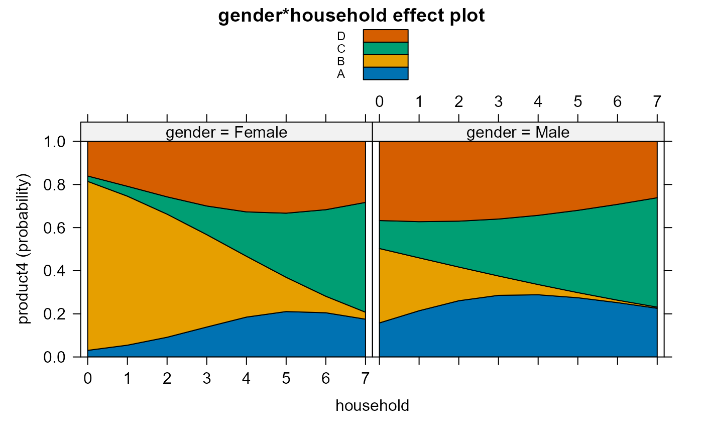
eff.gen.hh <- effects::Effect(c("gender", "household"), m.health,
xlevels=list(household=0:7))
eff.gen.hh
#>
#> gender*household effect (probability) for A
#> household
#> gender 0 1 2 3 4 5
#> Female 0.03068509 0.05472636 0.09144115 0.1388314 0.1849404 0.2106384
#> Male 0.15791974 0.21437570 0.26076677 0.2858916 0.2885194 0.2747927
#> household
#> gender 6 7
#> Female 0.2050717 0.1752920
#> Male 0.2521037 0.2259001
#>
#> gender*household effect (probability) for B
#> household
#> gender 0 1 2 3 4 5
#> Female 0.7838489 0.6912060 0.5710296 0.42865766 0.28233237 0.15899102
#> Male 0.3451940 0.2454767 0.1564209 0.08983625 0.04749338 0.02369578
#> household
#> gender 6 7
#> Female 0.07653266 0.032345146
#> Male 0.01138814 0.005345618
#>
#> gender*household effect (probability) for C
#> household
#> gender 0 1 2 3 4 5
#> Female 0.02488288 0.04580833 0.08031185 0.1328261 0.2057312 0.2973862
#> Male 0.12979288 0.16787840 0.21281420 0.2641723 0.3209620 0.3816852
#> household
#> gender 6 7
#> Female 0.4016088 0.5093355
#> Male 0.4444909 0.5073987
#>
#> gender*household effect (probability) for D
#> household
#> gender 0 1 2 3 4 5 6
#> Female 0.1605831 0.2082593 0.2572174 0.2996849 0.3269960 0.3329844 0.3167868
#> Male 0.3670934 0.3722692 0.3699982 0.3600999 0.3430252 0.3198263 0.2920173
#> household
#> gender 7
#> Female 0.2830274
#> Male 0.2613555
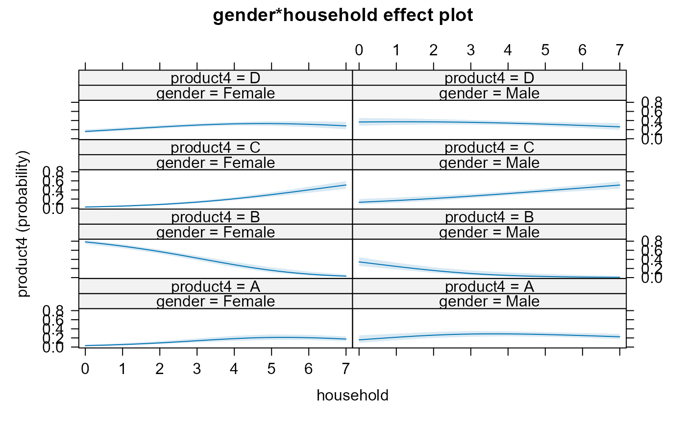
plot(eff.gen.hh, axes=list(x=list(rug=FALSE)))
summary(peff.women)
#>
#> hincome predictor effect
#>
#> hincome effect (probability) for not.work
#> hincome
#> 1 1.9 2.8 3.69 4.59 5.49 6.39 7.29
#> 0.4523534 0.4618023 0.4712788 0.4806704 0.4901814 0.4996996 0.5092179 0.5187296
#> 8.18 9.08 9.98 10.9 11.8 12.7 13.6 14.5
#> 0.5281223 0.5376003 0.5470512 0.5566771 0.5660528 0.5753815 0.5846568 0.5938724
#> 15.4 16.3 17.2 18.1 19 19.9 20.8 21.7
#> 0.6030225 0.6121010 0.6211024 0.6300212 0.6388520 0.6475901 0.6562304 0.6647686
#> 22.6 23.4 24.3 25.2 26.1 27 27.9 28.8
#> 0.6732003 0.6806026 0.6888224 0.6969250 0.7049069 0.7127653 0.7204974 0.7281007
#> 29.7 30.6 31.5 32.4 33.3 34.2 35.1 36
#> 0.7355732 0.7429127 0.7501178 0.7571869 0.7641189 0.7709129 0.7775682 0.7840843
#> 36.9 37.8 38.7 39.6 40.5 41.4 42.3 43.2
#> 0.7904609 0.7966981 0.8027959 0.8087547 0.8145751 0.8202576 0.8258033 0.8312131
#> 44.1 45
#> 0.8364881 0.8416297
#>
#> hincome effect (probability) for parttime
#> hincome
#> 1 1.9 2.8 3.69 4.59 5.49 6.39
#> 0.09864534 0.10359265 0.10854405 0.11368937 0.11877884 0.12400783 0.12915775
#> 7.29 8.18 9.08 9.98 10.9 11.8 12.7
#> 0.13440804 0.13956000 0.14473686 0.14972987 0.15465311 0.15983886 0.16389146
#> 13.6 14.5 15.4 16.3 17.2 18.1 19
#> 0.16883681 0.17249633 0.17698253 0.18015718 0.18408391 0.18669457 0.18997787
#> 19.9 20.8 21.7 22.6 23.4 24.3 25.2
#> 0.19289987 0.19453999 0.19673115 0.19769122 0.19970141 0.19998331 0.20067294
#> 26.1 27 27.9 28.8 29.7 30.6 31.5
#> 0.20028308 0.20024010 0.19982683 0.19848381 0.19741243 0.19551731 0.19385571
#> 32.4 33.3 34.2 35.1 36 36.9 37.8
#> 0.19147712 0.18930194 0.18651379 0.18390586 0.18078344 0.17782378 0.17470521
#> 38.7 39.6 40.5 41.4 42.3 43.2 44.1
#> 0.17120718 0.16785358 0.16419793 0.16067852 0.15692500 0.15330158 0.14950269
#> 45
#> 0.14582907
#>
#> hincome effect (probability) for fulltime
#> hincome
#> 1 1.9 2.8 3.69 4.59 5.49 6.39
#> 0.44900129 0.43460502 0.42017715 0.40564022 0.39103972 0.37629259 0.36162433
#> 7.29 8.18 9.08 9.98 10.9 11.8 12.7
#> 0.34686236 0.33231772 0.31766287 0.30321897 0.28866980 0.27410834 0.26072707
#> 13.6 14.5 15.4 16.3 17.2 18.1 19
#> 0.24650643 0.23363123 0.21999498 0.20774179 0.19481368 0.18328427 0.17117008
#> 19.9 20.8 21.7 22.6 23.4 24.3 25.2
#> 0.15951007 0.14922960 0.13850025 0.12910846 0.11969604 0.11119425 0.10240207
#> 26.1 27 27.9 28.8 29.7 30.6 31.5
#> 0.09480998 0.08699458 0.07967577 0.07341545 0.06701441 0.06156996 0.05602651
#> 32.4 33.3 34.2 35.1 36 36.9 37.8
#> 0.05133597 0.04657912 0.04257327 0.03852592 0.03513225 0.03171528 0.02859670
#> 38.7 39.6 40.5 41.4 42.3 43.2 44.1
#> 0.02599692 0.02339170 0.02122701 0.01906384 0.01727168 0.01548533 0.01400918
#> 45
#> 0.01254120
#>
#> Lower 95 Percent Confidence Limits for not.work
#> hincome
#> 1 1.9 2.8 3.69 4.59 5.49 6.39 7.29
#> 0.3159695 0.3310511 0.3463719 0.3617049 0.3773328 0.3930128 0.4086632 0.4241902
#> 8.18 9.08 9.98 10.9 11.8 12.7 13.6 14.5
#> 0.4393183 0.4542674 0.4687299 0.4828570 0.4958777 0.5079597 0.5189802 0.5288600
#> 15.4 16.3 17.2 18.1 19 19.9 20.8 21.7
#> 0.5375785 0.5451759 0.5517427 0.5574002 0.5622799 0.5665088 0.5702001 0.5734503
#> 22.6 23.4 24.3 25.2 26.1 27 27.9 28.8
#> 0.5763392 0.5786565 0.5810295 0.5831958 0.5851899 0.5870396 0.5887674 0.5903915
#> 29.7 30.6 31.5 32.4 33.3 34.2 35.1 36
#> 0.5919270 0.5933862 0.5947793 0.5961148 0.5974000 0.5986407 0.5998422 0.6010089
#> 36.9 37.8 38.7 39.6 40.5 41.4 42.3 43.2
#> 0.6021445 0.6032522 0.6043348 0.6053948 0.6064343 0.6074552 0.6084592 0.6094476
#> 44.1 45
#> 0.6104217 0.6113828
#>
#> Lower 95 Percent Confidence Limits for parttime
#> hincome
#> 1 1.9 2.8 3.69 4.59 5.49 6.39
#> 0.03847131 0.04276604 0.04735083 0.05237580 0.05766875 0.06338466 0.06932277
#> 7.29 8.18 9.08 9.98 10.9 11.8 12.7
#> 0.07562710 0.08206002 0.08872208 0.09531895 0.10190947 0.10865531 0.11405577
#> 13.6 14.5 15.4 16.3 17.2 18.1 19
#> 0.12001554 0.12428948 0.12878012 0.13151369 0.13424863 0.13536112 0.13643431
#> 19.9 20.8 21.7 22.6 23.4 24.3 25.2
#> 0.13676393 0.13586219 0.13501729 0.13317007 0.13208517 0.12954146 0.12715419
#> 26.1 27 27.9 28.8 29.7 30.6 31.5
#> 0.12406951 0.12116163 0.11802865 0.11436509 0.11089064 0.10698659 0.10327582
#> 32.4 33.3 34.2 35.1 36 36.9 37.8
#> 0.09923212 0.09538532 0.09129674 0.08740835 0.08336110 0.07951628 0.07571321
#> 38.7 39.6 40.5 41.4 42.3 43.2 44.1
#> 0.07185586 0.06820070 0.06454437 0.06108654 0.05766792 0.05444130 0.05128269
#> 45
#> 0.04830710
#>
#> Lower 95 Percent Confidence Limits for fulltime
#> hincome
#> 1 1.9 2.8 3.69 4.59 5.49
#> 0.311275740 0.303984689 0.296573453 0.288937743 0.281161091 0.273127893
#> 6.39 7.29 8.18 9.08 9.98 10.9
#> 0.264972521 0.256539050 0.247988764 0.239080389 0.229964345 0.220368072
#> 11.8 12.7 13.6 14.5 15.4 16.3
#> 0.210239105 0.200459222 0.189418729 0.178861142 0.167036383 0.155895357
#> 17.2 18.1 19 19.9 20.8 21.7
#> 0.143650271 0.132406067 0.120351187 0.108642000 0.098350645 0.087704592
#> 22.6 23.4 24.3 25.2 26.1 27
#> 0.078576692 0.069613542 0.061804111 0.053997739 0.047553785 0.041196107
#> 27.9 28.8 29.7 30.6 31.5 32.4
#> 0.035543805 0.030976068 0.026541740 0.022997990 0.019587626 0.016887733
#> 33.3 34.2 35.1 36 36.9 37.8
#> 0.014308889 0.012283444 0.010361274 0.008861644 0.007446381 0.006245988
#> 38.7 39.6 40.5 41.4 42.3 43.2
#> 0.005317145 0.004446673 0.003775970 0.003149807 0.002669044 0.002221675
#> 44.1 45
#> 0.001879189 0.001561390
#>
#> Upper 95 Percent Confidence Limits for not.work
#> hincome
#> 1 1.9 2.8 3.69 4.59 5.49 6.39 7.29
#> 0.5962883 0.5980285 0.5998890 0.6018689 0.6040398 0.6064137 0.6090323 0.6119467
#> 8.18 9.08 9.98 10.9 11.8 12.7 13.6 14.5
#> 0.6151814 0.6188841 0.6231101 0.6280763 0.6336758 0.6401102 0.6474575 0.6557532
#> 15.4 16.3 17.2 18.1 19 19.9 20.8 21.7
#> 0.6649766 0.6750482 0.6858407 0.6971996 0.7089624 0.7209753 0.7331010 0.7452227
#> 22.6 23.4 24.3 25.2 26.1 27 27.9 28.8
#> 0.7572438 0.7677810 0.7794113 0.7907560 0.8017765 0.8124433 0.8227350 0.8326368
#> 29.7 30.6 31.5 32.4 33.3 34.2 35.1 36
#> 0.8421394 0.8512380 0.8599317 0.8682226 0.8761155 0.8836175 0.8907373 0.8974849
#> 36.9 37.8 38.7 39.6 40.5 41.4 42.3 43.2
#> 0.9038717 0.9099097 0.9156116 0.9209906 0.9260599 0.9308333 0.9353240 0.9395456
#> 44.1 45
#> 0.9435113 0.9472341
#>
#> Upper 95 Percent Confidence Limits for parttime
#> hincome
#> 1 1.9 2.8 3.69 4.59 5.49 6.39 7.29
#> 0.2303876 0.2301342 0.2297475 0.2294036 0.2289148 0.2284694 0.2279869 0.2276258
#> 8.18 9.08 9.98 10.9 11.8 12.7 13.6 14.5
#> 0.2273707 0.2272957 0.2273933 0.2277713 0.2289403 0.2298530 0.2322760 0.2343960
#> 15.4 16.3 17.2 18.1 19 19.9 20.8 21.7
#> 0.2382923 0.2417837 0.2471379 0.2518255 0.2582505 0.2650038 0.2706237 0.2776004
#> 22.6 23.4 24.3 25.2 26.1 27 27.9 28.8
#> 0.2832578 0.2903517 0.2957168 0.3019922 0.3069096 0.3125739 0.3178821 0.3219802
#> 29.7 30.6 31.5 32.4 33.3 34.2 35.1 36
#> 0.3266412 0.3302172 0.3342662 0.3373568 0.3408474 0.3434981 0.3464878 0.3487438
#> 36.9 37.8 38.7 39.6 40.5 41.4 42.3 43.2
#> 0.3512872 0.3536093 0.3553357 0.3572844 0.3587123 0.3603271 0.3614863 0.3628022
#> 44.1 45
#> 0.3637196 0.3647681
#>
#> Upper 95 Percent Confidence Limits for fulltime
#> hincome
#> 1 1.9 2.8 3.69 4.59 5.49 6.39
#> 0.59501785 0.57498523 0.55467452 0.53407517 0.51320236 0.49204610 0.47094270
#> 7.29 8.18 9.08 9.98 10.9 11.8 12.7
#> 0.44974914 0.42896528 0.40821763 0.38804929 0.36814483 0.34881095 0.33159955
#> 13.6 14.5 15.4 16.3 17.2 18.1 19
#> 0.31413172 0.29906450 0.28401891 0.27128922 0.25869488 0.24812169 0.23765017
#> 19.9 20.8 21.7 22.6 23.4 24.3 25.2
#> 0.22810055 0.22000694 0.21188244 0.20490995 0.19813645 0.19197757 0.18568011
#> 26.1 27 27.9 28.8 29.7 30.6 31.5
#> 0.18014460 0.17444460 0.16900120 0.16415016 0.15911498 0.15459766 0.14988910
#> 32.4 33.3 34.2 35.1 36 36.9 37.8
#> 0.14564305 0.14120153 0.13718125 0.13296332 0.12913585 0.12511026 0.12117493
#> 38.7 39.6 40.5 41.4 42.3 43.2 44.1
#> 0.11759700 0.11382363 0.11039273 0.10676980 0.10347772 0.09999840 0.09684042
#> 45
#> 0.09350127
#> NULL
#>
#> children predictor effect
#>
#> children effect (probability) for not.work
#> children
#> absent present
#> 0.3292677 0.7035269
#>
#> children effect (probability) for parttime
#> children
#> absent present
#> 0.08765899 0.20178389
#>
#> children effect (probability) for fulltime
#> children
#> absent present
#> 0.58307330 0.09468924
#>
#> Lower 95 Percent Confidence Limits for not.work
#> children
#> absent present
#> 0.2339044 0.6329284
#>
#> Lower 95 Percent Confidence Limits for parttime
#> children
#> absent present
#> 0.0409294 0.1481547
#>
#> Lower 95 Percent Confidence Limits for fulltime
#> children
#> absent present
#> 0.4696612 0.0582675
#>
#> Upper 95 Percent Confidence Limits for not.work
#> children
#> absent present
#> 0.4411236 0.7655763
#>
#> Upper 95 Percent Confidence Limits for parttime
#> children
#> absent present
#> 0.1778469 0.2687024
#>
#> Upper 95 Percent Confidence Limits for fulltime
#> children
#> absent present
#> 0.6883270 0.1502452
#> NULL
dichots <- logits(AB_CD = dichotomy(c("A", "B"), c("C", "D")),
A_B = dichotomy("A", "B"),
C_D = dichotomy("C", "D"))
m.health <- nestedLogit(product4 ~ age + gender*household + position_level,
dichotomies = dichots, data = HealthInsurance)
eff.gen.hh <- effects::Effect(c("gender", "household"), m.health,
xlevels=list(household=0:7))
eff.gen.hh
#>
#> gender*household effect (probability) for A
#> household
#> gender 0 1 2 3 4 5
#> Female 0.03068509 0.05472636 0.09144115 0.1388314 0.1849404 0.2106384
#> Male 0.15791974 0.21437570 0.26076677 0.2858916 0.2885194 0.2747927
#> household
#> gender 6 7
#> Female 0.2050717 0.1752920
#> Male 0.2521037 0.2259001
#>
#> gender*household effect (probability) for B
#> household
#> gender 0 1 2 3 4 5
#> Female 0.7838489 0.6912060 0.5710296 0.42865766 0.28233237 0.15899102
#> Male 0.3451940 0.2454767 0.1564209 0.08983625 0.04749338 0.02369578
#> household
#> gender 6 7
#> Female 0.07653266 0.032345146
#> Male 0.01138814 0.005345618
#>
#> gender*household effect (probability) for C
#> household
#> gender 0 1 2 3 4 5
#> Female 0.02488288 0.04580833 0.08031185 0.1328261 0.2057312 0.2973862
#> Male 0.12979288 0.16787840 0.21281420 0.2641723 0.3209620 0.3816852
#> household
#> gender 6 7
#> Female 0.4016088 0.5093355
#> Male 0.4444909 0.5073987
#>
#> gender*household effect (probability) for D
#> household
#> gender 0 1 2 3 4 5 6
#> Female 0.1605831 0.2082593 0.2572174 0.2996849 0.3269960 0.3329844 0.3167868
#> Male 0.3670934 0.3722692 0.3699982 0.3600999 0.3430252 0.3198263 0.2920173
#> household
#> gender 7
#> Female 0.2830274
#> Male 0.2613555
plot(eff.gen.hh, axes=list(x=list(rug=FALSE)))
 plot(eff.gen.hh, axes=list(x=list(rug=FALSE),
y=list(style="stacked")))
plot(eff.gen.hh, axes=list(x=list(rug=FALSE),
y=list(style="stacked")))