Nested-dichotomies logistic regression models

Michael Friendly and John Fox

2023-08-05

Load the packages we’ll use here:

library(nestedLogit)    # Nested Dichotomy Logistic Regression Models
library(knitr)          # A General-Purpose Package for Dynamic Report Generation in R
library(car)            # Companion to Applied Regression
library(nnet)           # Feed-Forward Neural Networks and Multinomial Log-Linear Models
library(broom)          # Convert Statistical Objects into Tidy Tibbles
library(dplyr)          # A Grammar of Data Manipulation
library(effects)        # Effect Displays for Linear, Generalized Linear, and Other Models

Models for polytomous responses

The familiar logistic-regression model applies when there is a binary (“dichotomous”) response, such as “survived” vs. “died”, or voted “yes” vs. “no” on a referendum. Often, however, the response variable is multi-category (“polytomous”), taking on \(m > 2\) discrete values. For example,

• Respondents to a social survey are classified by their highest completed level of education, taking on the values (1) less than highschool, (2) highschool graduate, (3) some post-secondary, or (4) post-secondary degree.

• Women’s labor-force participation is classified as (1) not working outside the home, (2) working part-time, or (3) working full-time.

• Voters in Quebec in a Canadian national election choose one of the (1) Liberal Party, (2) Conservative Party, (3) New Democratic Party, or (4) Bloc Quebecois.

The numbers in these examples, (1), (2), etc., are category labels, and the categories may be ordered (as in the first two examples) or may not (as in the third).

There are several different ways to model the category probabilities for a polytomous response. Let \(\phi_{ij} \equiv \phi_j \, ( \vec{x}_i )\) be the probability of response \(j\) for case \(i\), given the predictors \(\vec{x}_i\). Because \(\sum_j \, \phi_{ij} = 1\), any \(m - 1\) of these probabilities imply the last; for example, \(\phi_{im} = 1 - \sum_{j = 1}^{m - 1} \, \phi_{ij}\). The essential idea is to construct a model for the polytomous response composed of \(m-1\) logit comparisons among the response categories in a manner analogous to to the treatment of factors in the predictor variables. There are also more restrictive models specifically for ordered categorical responses, but we will not consider them here.

Multinomial logit model

One natural generalization of the the standard logistic-regression (or logit) model is the multinomial logit (or generalized logit) model. When the polytomous response has \(m\) levels, the multinomial logit model comprises \(m-1\) log-odds comparisons with a reference level, typically the first or last, as described in Fox (2016, sec. 14.2.1) and Friendly & Meyer (2016, sec. 8.3). This is an inessential choice, in that the likelihood under the model and the fitted response probabilities that it produces are unaffected by choice of reference level, much as choice of reference level for dummy regressors created from a factor predictor doesn’t affect the fit of a regression model. The standard implementation of this model in R is multinom() in the nnet package (Venables & Ripley, 2002), which takes the first level of the response as the omitted reference category.

Nested-dichotomies logit model

Because it uses the familiar dichotomous logit model, fitting separate models for each of a hierarchically nested set of binary comparisons among the response categories, the nested-dichotomies logit model can be a simpler alternative to the multinomial logit model. Standard methods for model summaries, tests and graphs can then be employed for each of the constituent binary logit models, and taken together, the set of \(m-1\) models comprises a complete model for the polytomous response, just as the multinomial logit model does. This approach is described by Fienberg (1980) and is also discussed by Fox (2016, sec. 14.2.2) and Friendly & Meyer (2016, sec. 8.2).

For an \(m\)-category response and a model-matrix with \(p\) regressors, both the nested-dichotomies logit model and the multinomial logit model have \(p \times (m - 1)\) parameters. The models are not equivalent, however, in that they generally produce different sets of fitted category probabilities and hence different likelihoods.

By the construction of nested dichotomies, the submodels are statistically independent (because the likelihood for the polytomous response is the product of the likelihoods for the dichotomies), so test statistics, such as likelihood ratio (\(G^2\)) and Wald chi-square tests for regression coefficients can be summed to give overall tests for the full polytomy. In this way, the \(m-1\) dichotomies are analogous to \(m-1\) orthogonal contrasts for an \(m\)-level factor in a balanced ANOVA design.

Alternative sets of nested dichotomies are illustrated in the figure below, for a four-category polytomous response response \(Y = \{1, 2, 3, 4\}\). In the case shown at the left of the figure, the response categories are divided first as \(\{1, 2\}\) vs. \(\{3, 4\}\). Then these compound categories are subdivided as the dichotomies \(\{1\}\) vs. \(\{2\}\) and as \(\{3\}\) vs. \(\{4\}\). Alternatively, as shown at the right of the figure, the response categories are divided progressively: first as \(\{1\}\) vs. \(\{2, 3, 4\}\); next as \(\{2\}\) vs. \(\{3, 4\}\); and and finally \(\{3\}\) vs. \(\{4\}\).

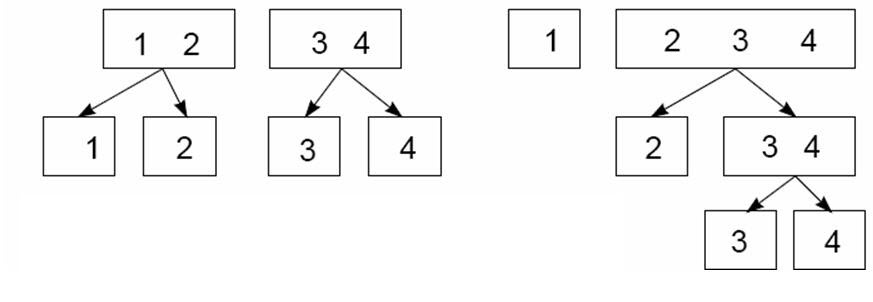
Nested dichotomies: The boxes show two different ways a four-category response can be represented as three nested dichotomies.

This example makes clear that nested dichotomies are not unique and that alternative sets of nested dichotomies are not equivalent: Different choices have different interpretations. Moreover, and more fundamentally, fitted probabilities and hence the likelihood for the nested-dichotomies model depend on how the nested dichotomies are defined.

The nested-dichotomies model is consequently most compelling when there is a natural and unique way to define the dichotomies, such as a process that proceeds through an orderly sequence of stages. Consider the set of nested dichotomies at the right of the figure above, and the previously mentioned four-level educational response variable with categories (1) less than highschool, (2) highschool graduate, (3) some post-secondary, and (4) post-secondary degree. In the vast majority of cases, individuals proceed through these educational stages in sequence. The first dichotomy, \(\{1\}\) vs. \(\{2, 3, 4\}\), therefore represents highschool graduation; the second, \(\{2\}\) vs. \(\{3, 4\}\), enrollment in post-secondary education; and the third, \(\{3\}\) vs. \(\{4\}\), completion of a post-secondary degree. This scheme for generating the logits for the nested-dichotomies model is termed continuation logits.

To take another example, the figure below shows the classification of psychiatric patients into four diagnostic categories. These might be naturally dichotomized by contrasting the normal individuals to the groups of patients, and then dividing the patient groups into a comparison of depressed and manic patients vs. schizophrenics, followed by a comparison of depressed vs. manic patients. A model predicting diagnosis can be interpreted in terms of the probabilities of classification into each of the response categories.

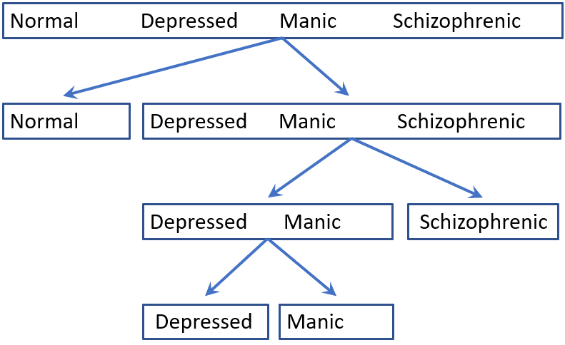
Psychiatric classification: The figure shows how four diagnostic categories might be represented by nested dichotomies.

Example: Women’s labor-force participation

For a principal example, we consider the data set Womenlf from the carData package (Fox, Weisberg, & Price, 2022). The data give the responses of 263 young married women, 21–30 years old, drawn from a 1977 survey carried out by the York University Institute for Social Research (Atkinson, Blishen, Ornstein, & Stevenson, 1984). This example was originally developed by Fox (1984, sec. 5.1.5). The variables in the model are:

• partic: labor force participation, the response, with levels:
  • "fulltime": working full-time
  • "not.work": not working outside the home
  • "parttime" : working part-time.
• hincome: Husband’s income, in $1,000s.
• children: Presence of children in the home, "absent" or "present".
• region: Region of Canada (“Atlantic”, “BC”, “Ontario”, “Prairie”, “Quebec”).

The response, partic is a factor, but the levels are ordered alphabetically. To facilitate interpretation, we reorder the levels of partic:

data(Womenlf, package = "carData")
Womenlf$partic <- with(Womenlf, 
                       factor(partic, levels = c("not.work", "parttime", "fulltime")))

In 1977, the majority of the 263 women in the sample were not working outside the home:

xtabs(~ partic, data=Womenlf)
#> partic
#> not.work parttime fulltime 
#>      155       42       66

Defining nested dichotomies

How can we understand these womens’ labor-force participation choices in terms of the explanatory variables? We’ll consider three polytomous logit models for the Womenlf data, two of which entail different choices of nested dichotomies, and the multinomial logit model. The example will illustrate the potential pitfalls and advantages of the nested-dichotomies approach in a context where there isn’t a compelling choice of nested dichotomies.

It is at least arguable to construe a woman’s labor-force choice as first involving a dichotomy (let’s call it work) between women who are not working outside the home vs. those who are working (either part-time or full-time). A second dichotomy (full) contrasts those who work full-time time vs. part-time, but among only those who work.

The two binary variables for the nested dichotomies can be created by recoding partic as follows.

Womenlf <- within(Womenlf, {
  work = ifelse(partic == "not.work", 0, 1)
  full = ifelse(partic == "fulltime",  1,
                ifelse(partic == "parttime", 0, NA))
})

Note that the complete sample of 263 cases is available for the work dichotomy, while only 108 cases—excluding those not working outside the home—are available for the full dichotomy:

xtabs(~ work, data=Womenlf)
#> work
#>   0   1 
#> 155 108
xtabs(~ full, data=Womenlf, addNA=TRUE)
#> full
#>    0    1 <NA> 
#>   42   66  155

The relationship of the response variable partic to the two nested dichotomies is as follows:

xtabs(~ partic + work, data=Womenlf)
#>           work
#> partic       0   1
#>   not.work 155   0
#>   parttime   0  42
#>   fulltime   0  66
xtabs(~ partic + full, addNA=TRUE, data=Womenlf)
#>           full
#> partic       0   1 <NA>
#>   not.work   0   0  155
#>   parttime  42   0    0
#>   fulltime   0  66    0

We can then fit separate binary logit models to the two nested dichotomies directly:

mod.work <- glm(work ~ hincome + children, family=binomial, data=Womenlf)
mod.full <- glm(full ~ hincome + children, family=binomial, data=Womenlf)

In equation form, the two log-odds models are shown below. (Model equations are conveniently rendered in markdown/LaTeX using the equatiomatic package (Anderson, Heiss, & Sumners, 2023).)

\[ L_1 =\log\left[ \frac { P( \operatorname{work} = \operatorname{1} ) }{ 1 - P( \operatorname{work} = \operatorname{1} ) } \right] = \alpha_1 + \beta_{11}(\operatorname{hincome}) + \beta_{12}(\operatorname{children}_{\operatorname{present}}) \] \[ L_2 = \log\left[ \frac { P( \operatorname{full} ) }{ 1 - P( \operatorname{full} ) } \right] = \alpha_2 + \beta_{21}(\operatorname{hincome}) + \beta_{22}(\operatorname{children}_{\operatorname{present}}) \] The estimated regression coefficients for the two binary logit models are

mod.work
#> 
#> Call:  glm(formula = work ~ hincome + children, family = binomial, data = Womenlf)
#> 
#> Coefficients:
#>     (Intercept)          hincome  childrenpresent  
#>          1.3358          -0.0423          -1.5756  
#> 
#> Degrees of Freedom: 262 Total (i.e. Null);  260 Residual
#> Null Deviance:       356 
#> Residual Deviance: 320   AIC: 326
mod.full
#> 
#> Call:  glm(formula = full ~ hincome + children, family = binomial, data = Womenlf)
#> 
#> Coefficients:
#>     (Intercept)          hincome  childrenpresent  
#>           3.478           -0.107           -2.651  
#> 
#> Degrees of Freedom: 107 Total (i.e. Null);  105 Residual
#>   (155 observations deleted due to missingness)
#> Null Deviance:       144 
#> Residual Deviance: 104   AIC: 110

A disadvantage of this approach is that it is tedious to obtain tests for the combined model, to compute and plot predicted probabilities, and so forth.

Using dichotomy() and logits() to define the response

Instead, the nestedLogit package provides tools to specify and manipulate the nested-logit model. The dichotomy() function defines a single dichotomy, and the logits() function uses \(m-1\) calls to dichotomy() to create a "dichotomies" object representing the nested dichotomies. For example:

comparisons <- logits(work=dichotomy("not.work", working=c("parttime", "fulltime")),
                      full=dichotomy("parttime", "fulltime"))

comparisons
#> work: {not.work} vs. working{parttime, fulltime}
#> full: {parttime} vs. {fulltime}

It is mandatory to name the dichotomies (here work and full), and we can optionally name the elements of each dichotomy, an option that is particularly useful for a compound category, such as working=c("parttime", "fulltime") in the example.

There are coercion functions to convert the set of nested dichotomies to a matrix or to a character string, representing the tree structure of the dichotomies:

as.matrix(comparisons)
#>      not.work parttime fulltime
#> work        0        1        1
#> full       NA        0        1

cat(as.character(comparisons))
#> work = {{not.work}} {working{parttime fulltime}}; full = {{parttime}} {{fulltime}}

Using nestedLogit() to fit the model

To fit the model, we supply comparisons as the dichotomies argument to the nestedLogit() function. The model formula argument, partic ~ hincome + children specifies a main-effects model for husband’s income and presence of young children; aside from the dichotomies argument, the general format of the function call is typical for an R statistical modeling function (with optional subset and contrasts arguments not shown in this example). An atypical feature of nestedLogit() is that the data argument is required.

wlf.nested <- nestedLogit(partic ~ hincome + children, 
                          dichotomies = comparisons,
                          data=Womenlf)

The result, wlf.nested, is a an object of class "nestedLogit", encapsulating the details of the model for the nested dichotomies. The models component of the object contains essentially the same "glm" model objects as we constructed directly as mod.work and mod.full above, here named work and full.

names(wlf.nested)
#> [1] "models"          "formula"         "dichotomies"     "data"           
#> [5] "data.name"       "subset"          "contrasts"       "contrasts.print"

names(wlf.nested$models) # equivalent: names(models(wlf.models))
#> [1] "work" "full"

# view the separate models
models(wlf.nested, 1) 
#> 
#> Call:  glm(formula = work ~ hincome + children, family = binomial, data = Womenlf, 
#>     contrasts = contrasts)
#> 
#> Coefficients:
#>     (Intercept)          hincome  childrenpresent  
#>          1.3358          -0.0423          -1.5756  
#> 
#> Degrees of Freedom: 262 Total (i.e. Null);  260 Residual
#> Null Deviance:       356 
#> Residual Deviance: 320   AIC: 326

models(wlf.nested, 2)
#> 
#> Call:  glm(formula = full ~ hincome + children, family = binomial, data = Womenlf, 
#>     contrasts = contrasts)
#> 
#> Coefficients:
#>     (Intercept)          hincome  childrenpresent  
#>           3.478           -0.107           -2.651  
#> 
#> Degrees of Freedom: 107 Total (i.e. Null);  105 Residual
#>   (155 observations deleted due to missingness)
#> Null Deviance:       144 
#> Residual Deviance: 104   AIC: 110

Methods for "nestedLogit" objects

As befits a model-fitting function, the package defines a nearly complete set of methods for "nestedLogit" objects:

• print() and summary() print the results for each of the submodels.
• update() re-fits the model, allowing changes to the model formula, data, subset, and contrasts arguments.
• coef() returns the coefficients for the predictors in each dichotomy.
• vcov() returns the variance-covariance matrix of the coefficients
• predict() computes predicted probabilities for the response categories, either for the cases in the data, which is equivalent to fitted(), or for arbitrary combinations of the predictors; the latter is useful for producing plots to aid interpretation.
• confint() calculates confidence intervals for the predicted probabilities or predicted logits.
• as.data.frame() method for predicted probabilities and logits converts these to long format for use with ggplot2.
• glance() and tidy() are extensions of broom::glance.glm() and broom::tidy.glm() to obtain compact summaries of a "nestedLogit" model object.
• plot() provides basic plots of the predicted probabilities over a range of values of the predictor variables.
• models() is an extractor function for the binary logit models in the "nestedLogit" object
• Effect() calculates marginal effects collapsed over some variable(s) for the purpose of making effect plots.

These functions are supplemented by various methods for testing hypotheses about and comparing nested-logit models:

• anova() provides analysis-of-deviance Type I (sequential) tests for each dichotomy and for the combined model. When given a sequence of model objects, anova() tests the models against one another in the order specified.
• Anova() uses car::Anova() to provide analysis-of-deviance Type II or III (partial) tests for each dichotomy and for the combined model.
• linearHypothesis() uses car::linearHypothesis() to compute Wald tests for hypotheses about coefficients or their linear combinations.
• logLik() returns the log-likelihood and degrees of freedom for the nested-dichotomies logit model.
• Through logLik(), the AIC() and BIC() functions compute the Akaike and Bayesian information criteria model-comparison statistics.

We illustrate the application of some of these methods:

Coefficients: By default, coef() returns a matrix whose rows are the regressors in the model and whose columns represent the nested dichotomies. In the Womenlf example, the coefficients \(\widehat{\beta}_{j1}\) give the estimated change in the log-odds of working vs. not working associated with a $1,000 increase in husband’s income and with having children present vs. absent, each holding the other constant. The coefficients \(\widehat{\beta}_{j2}\) are similar for the log-odds of working full-time vs. part-time among those who are working outside the home. The exponentiated coefficients \(e^{\widehat{\beta}_{jk}}\) give multiplicative effects on the odds for these comparisons.

coef(wlf.nested)
#>                     work    full
#> (Intercept)      1.33583  3.4778
#> hincome         -0.04231 -0.1073
#> childrenpresent -1.57565 -2.6515

# show as odds ratios
exp(coef(wlf.nested))
#>                   work     full
#> (Intercept)     3.8032 32.38753
#> hincome         0.9586  0.89829
#> childrenpresent 0.2069  0.07055

Thus, the odds of both working and working full-time decrease with husband’s income, by about 4% and 10% respectively per $1000. Having young children also decreases the odds of both working and working full-time, by about 79% and 93% respectively.

Analysis of deviance: A method for the Anova() function from the car package (Fox, Weisberg, & Price, 2023) computes Type II or III likelihood-ratio or Wald tests for each term in the model. Note that the likelihood-ratio or Wald \(\chi^2\) and degrees of freedom for the Combined Responses is the sum of their values for the separate dichotomies:

Anova(wlf.nested)
#> 
#>  Analysis of Deviance Tables (Type II tests)
#>  
#> Response work: {not.work} vs. working{parttime, fulltime}
#>          LR Chisq Df Pr(>Chisq)    
#> hincome      4.83  1      0.028 *  
#> children    31.32  1    2.2e-08 ***
#> ---
#> Signif. codes:  0 '***' 0.001 '**' 0.01 '*' 0.05 '.' 0.1 ' ' 1
#> 
#> 
#> Response full: {parttime} vs. {fulltime}
#>          LR Chisq Df Pr(>Chisq)    
#> hincome       9.0  1     0.0027 ** 
#> children     32.1  1    1.4e-08 ***
#> ---
#> Signif. codes:  0 '***' 0.001 '**' 0.01 '*' 0.05 '.' 0.1 ' ' 1
#> 
#> 
#> Combined Responses
#>          LR Chisq Df Pr(>Chisq)    
#> hincome      13.8  2      0.001 ** 
#> children     63.5  2    1.7e-14 ***
#> ---
#> Signif. codes:  0 '***' 0.001 '**' 0.01 '*' 0.05 '.' 0.1 ' ' 1

Linear hypotheses: The linearHypothesis() function in the car package provides a very general method for computing Wald tests of specific hypotheses about individual coefficients in a model or their linear combinations.

For example, the following command tests the hypothesis that the coefficients for hincome and children are simultaneously all equal to zero. This is equivalent to the test of the global null model, \(H_0\): all \(\beta_{jk} = 0\) for \(j = 1,2; k=1,2\) against an alternative that one or more coefficients \(\beta_{jk} \ne 0\).

linearHypothesis() reports this test for each of the submodels for the dichotomies work and full, as well as for the combined model:

linearHypothesis(wlf.nested, c("hincome", "childrenpresent"))
#> Linear hypothesis test
#> 
#> Hypothesis: 
#> hincome = 0 
#> childrenpresent = 0 
#>  
#> Model 1: restricted model
#> Model 2: partic ~ hincome + children 
#>  
#> Response work: {not.work} vs. working{parttime, fulltime} 
#>   Res.Df Df Chisq Pr(>Chisq)    
#> 1    262                        
#> 2    260  2  32.2      1e-07 ***
#> ---
#> Signif. codes:  0 '***' 0.001 '**' 0.01 '*' 0.05 '.' 0.1 ' ' 1
#> 
#> Response full: {parttime} vs. {fulltime}
#>   Res.Df Df Chisq Pr(>Chisq)    
#> 1    107                        
#> 2    105  2  25.6    2.8e-06 ***
#> ---
#> Signif. codes:  0 '***' 0.001 '**' 0.01 '*' 0.05 '.' 0.1 ' ' 1
#> 
#> Combined Responses
#> Chisq = 57.813, Df = 4, Pr(>Chisq) = 8.4e-12

Tidy summaries: The broom package (Robinson, Hayes, & Couch, 2023) provides functions for compact and tidy summaries of fitted models. The glance() method for a "nestedLogit" model produces a one-line summary of the statistics for each dichotomy. The tidy() method combines the coefficients for the sub-models, together with test statistics:

glance(wlf.nested)   # summarize the sub-models
#> # A tibble: 2 × 9
#>   response null.deviance df.null logLik   AIC   BIC deviance df.residual  nobs
#>   <chr>            <dbl>   <int>  <dbl> <dbl> <dbl>    <dbl>       <int> <int>
#> 1 work              356.     262 -160.   326.  336.     320.         260   263
#> 2 full              144.     107  -52.2  110.  119.     104.         105   108

tidy(wlf.nested)     # summarize the coefficients
#> # A tibble: 6 × 6
#>   response term            estimate std.error statistic      p.value
#>   <chr>    <chr>              <dbl>     <dbl>     <dbl>        <dbl>
#> 1 work     (Intercept)       1.34      0.384       3.48 0.000500    
#> 2 work     hincome          -0.0423    0.0198     -2.14 0.0324      
#> 3 work     childrenpresent  -1.58      0.292      -5.39 0.0000000700
#> 4 full     (Intercept)       3.48      0.767       4.53 0.00000580  
#> 5 full     hincome          -0.107     0.0392     -2.74 0.00615     
#> 6 full     childrenpresent  -2.65      0.541      -4.90 0.000000957

These functions facilitate the construction of custom tables. For example, to extract the likelihood-ratio difference-in-deviance (\(G^2\)) tests and compute (\(G^2 / df\)):

gl <- glance(wlf.nested)
gl |> 
  select(response, deviance, df.residual) |> 
  add_row(response = "Combined", deviance = sum(gl$deviance), df.residual = sum(gl$df.residual)) |>
  mutate(
    `P-value` = pchisq(deviance, df.residual, lower.tail = FALSE),
    `$G^2$/df` = deviance / df.residual) |>
  rename(`$G^2$` = deviance,
         df = df.residual) |>
  knitr::kable(digits = 3)

response	\(G^2\)	df	P-value	\(G^2\)/df
work	319.7	260	0.007	1.230
full	104.5	105	0.496	0.995
Combined	424.2	365	0.018	1.162

Model updating: The update() function makes it easy to create a new model from an old one, by adding or subtracting terms from the model formula, specifying a new formula, or changing the observations used or contrasts for factors.

For example, you might ask, “Does it make sense to include region of Canada in the model for the Womenlf data?” This question can be answered by adding region to the model formula, and comparing the new model to the original one using anova(). The tests here are for the additional contribution of region over and above the main effects of hincome and children:

wlf.nested.1 <- update(wlf.nested, formula = . ~ . + region)

anova(wlf.nested, wlf.nested.1)
#> 
#>  Analysis of Deviance Tables
#>  Model 1: partic ~ hincome + children
#>  Model 2: partic ~ hincome + children + region 
#>  
#> Response work: {not.work} vs. working{parttime, fulltime}
#>   Resid. Df Resid. Dev Df Deviance Pr(>Chi)
#> 1       260        320                     
#> 2       256        317  4     2.43     0.66
#> 
#> 
#> Response full: {parttime} vs. {fulltime}
#>   Resid. Df Resid. Dev Df Deviance Pr(>Chi)
#> 1       105        104                     
#> 2       101        102  4     2.65     0.62
#> 
#> 
#> Combined Responses
#>   Resid. Df Resid. Dev Df Deviance Pr(>Chi)
#> 1       365        424                     
#> 2       357        419  8     5.08     0.75

Recall that anova() with two or models tests the models sequentially against one another, in the order specified. This assumes that the models compared are nested (an unintentional pun), in the sense that the terms in the smaller model in each sequential pair are a subset of those in the larger model.

In a similar manner, we could fit and test a wider scope of models. For example to add an interaction between husband’s income and children and then test the interaction term:

wlf.nested.2 <- update(wlf.nested, formula = . ~ .^2)

anova(wlf.nested, wlf.nested.2)
#> 
#>  Analysis of Deviance Tables
#>  Model 1: partic ~ hincome + children
#>  Model 2: partic ~ hincome + children + hincome:children 
#>  
#> Response work: {not.work} vs. working{parttime, fulltime}
#>   Resid. Df Resid. Dev Df Deviance Pr(>Chi)
#> 1       260        320                     
#> 2       259        319  1    0.608     0.44
#> 
#> 
#> Response full: {parttime} vs. {fulltime}
#>   Resid. Df Resid. Dev Df Deviance Pr(>Chi)
#> 1       105        104                     
#> 2       104        104  1    0.256     0.61
#> 
#> 
#> Combined Responses
#>   Resid. Df Resid. Dev Df Deviance Pr(>Chi)
#> 1       365        424                     
#> 2       363        423  2    0.864     0.65

We can see that neither region nor the hincome \(\times\) children interaction make a difference to the fit either of the sub-models or of the combined model for the three response categories.

Obtaining fitted values: predict()

By default, predict() for a "nestedLogit" model object returns a "predictNestedLogit" object, which is a named list of four data frames whose columns are the response categories:

• p: predicted response-category probabilities.
• logit: the predicted probabilities transformed to the log-odds (logit) scale, logit = log(p / (1 - p)).
• se.p: standard errors of the predicted probabilities, computed by the delta method (see the corresponding vignette).
• se.logit: standard errors of the logits.

The computation is a bit tricky, because the probabilities of working full-time or part-time are conditional on working outside the home, but predict() takes care of the details. See vignette("standard-errors") for how these are calculated.

wlf.pred <- predict(wlf.nested)
print(wlf.pred, n=5)
#> 
#> First 5 of 263 rows:
#> 
#> predicted response-category probabilties
#>   not.work parttime fulltime
#> 1   0.7057   0.2020 0.092343
#> 2   0.6878   0.1993 0.112912
#> 3   0.8951   0.1030 0.001886
#> 4   0.7708   0.1920 0.037208
#> 5   0.7396   0.2007 0.059742
#>   . . .
#> 
#> predicted response-category logits
#>   not.work parttime fulltime
#> 1   0.8744   -1.374   -2.285
#> 2   0.7898   -1.391   -2.061
#> 3   2.1437   -2.164   -6.272
#> 4   1.2129   -1.437   -3.253
#> 5   1.0437   -1.382   -2.756
#>   . . .
#> 
#> standard errors of predicted probabilities
#>   not.work parttime fulltime
#> 1  0.03394  0.03077 0.022756
#> 2  0.03514  0.03104 0.024934
#> 3  0.05948  0.05846 0.002676
#> 4  0.04243  0.03908 0.017651
#> 5  0.03651  0.03368 0.020323
#>   . . .
#> 
#> standard errors of predicted logits
#>   not.work parttime fulltime
#> 1   0.1634   0.1909   0.2715
#> 2   0.1637   0.1945   0.2489
#> 3   0.6333   0.6326   1.4215
#> 4   0.2402   0.2519   0.4927
#> 5   0.1896   0.2100   0.3618
#>   . . .

By default, fitted values and standard errors are computed for all the observations in the data set. You can provide a newdata data.frame containing arbitrary combinations of predicted values, for example to obtain a grid of predicted values for custom plots or other purposes.

new <- expand.grid(hincome=seq(0, 45, length=4),
                   children=c("absent", "present"))

wlf.new <- predict(wlf.nested, new)

For greater flexibility, the as.data.frame() method for "predictNestedLogit" converts the components to long format.

as.data.frame(wlf.new) 
#>    hincome children response        p     se.p    logit se.logit
#> 1        0   absent not.work 0.208197 0.063264 -1.33583   0.3838
#> 2        0   absent parttime 0.023716 0.017749 -3.71762   0.7666
#> 3        0   absent fulltime 0.768088 0.063856  1.19755   0.3585
#> 4       15   absent not.work 0.331545 0.053684 -0.70120   0.2422
#> 5       15   absent parttime 0.089363 0.033557 -2.32144   0.4124
#> 6       15   absent fulltime 0.579092 0.056899  0.31905   0.2334
#> 7       30   absent not.work 0.483362 0.095465 -0.06658   0.3823
#> 8       30   absent parttime 0.224959 0.095639 -1.23700   0.5485
#> 9       30   absent fulltime 0.291679 0.101606 -0.88724   0.4918
#> 10      45   absent not.work 0.638313 0.147769  0.56805   0.6401
#> 11      45   absent parttime 0.287184 0.137011 -0.90910   0.6693
#> 12      45   absent fulltime 0.074503 0.077020 -2.51949   1.1170
#> 13       0  present not.work 0.559669 0.079322  0.23982   0.3219
#> 14       0  present parttime 0.134047 0.057151 -1.86564   0.4923
#> 15       0  present fulltime 0.306284 0.075679 -0.81755   0.3562
#> 16      15  present not.work 0.705670 0.033942  0.87445   0.1634
#> 17      15  present parttime 0.201988 0.030774 -1.37392   0.1909
#> 18      15  present fulltime 0.092343 0.022756 -2.28536   0.2715
#> 19      30  present not.work 0.818924 0.052611  1.50907   0.3548
#> 20      30  present parttime 0.165901 0.049356 -1.61496   0.3567
#> 21      30  present fulltime 0.015175 0.011492 -4.17279   0.7689
#> 22      45  present not.work 0.895078 0.059478  2.14370   0.6333
#> 23      45  present parttime 0.103036 0.058460 -2.16394   0.6326
#> 24      45  present fulltime 0.001886 0.002676 -6.27153   1.4215

Plotting "nestedLogit" objects

The nestedLogit package includes a basic plot() method for "nestedLogit" models, which calculates fitted probabilities and standard errors for the response categories and plots the probabilities and point-wise confidence limits against a single explanatory variable on the horizontal axis, while other explanatory variables are fixed to particular values. To produce multi-panel plots, it is necessary to call plot() repeatedly for various levels of the other predictors, and to compose these into a single figure, for example using par("mfcol"):

op <- par(mfcol=c(1, 2), mar=c(4, 4, 3, 1) + 0.1)
col <- scales::hue_pal()(3)                  # ggplot discrete colors
plot(wlf.nested, "hincome",                  # left panel
     other = list(children="absent"),
     xlab = "Husband's Income", 
     legend.location="top", col = col)
plot(wlf.nested, "hincome",                  # right panel
     other = list(children="present"),
     xlab = "Husband's Income", 
     legend=FALSE, col = col)
par(op)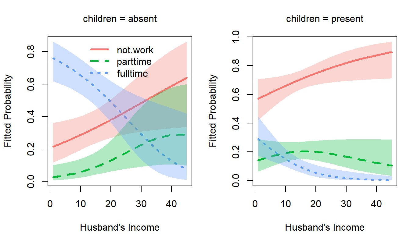

plot method: Predicted probabilities and 95 percent pointwise confidence envelopes of not working, working part-time, and working full-time

Effect plots for "nestedLogit" models

We provide a "nestedLogit" method for the Effect() function in the effects package (Fox, 2003; Fox & Weisberg, 2019). Because Effect() is the basic building block for other functions in the effects package, such as predictorEffects() (Fox & Weisberg, 2018), the full range of capabilities of the effects package is available; in particular, it’s possible to produce effect plots similar to those for multinomial logistic regression models (Fox & Hong, 2009).

We illustrate with the nested-logit model fit to the Womenlf data set:

plot(predictorEffects(wlf.nested))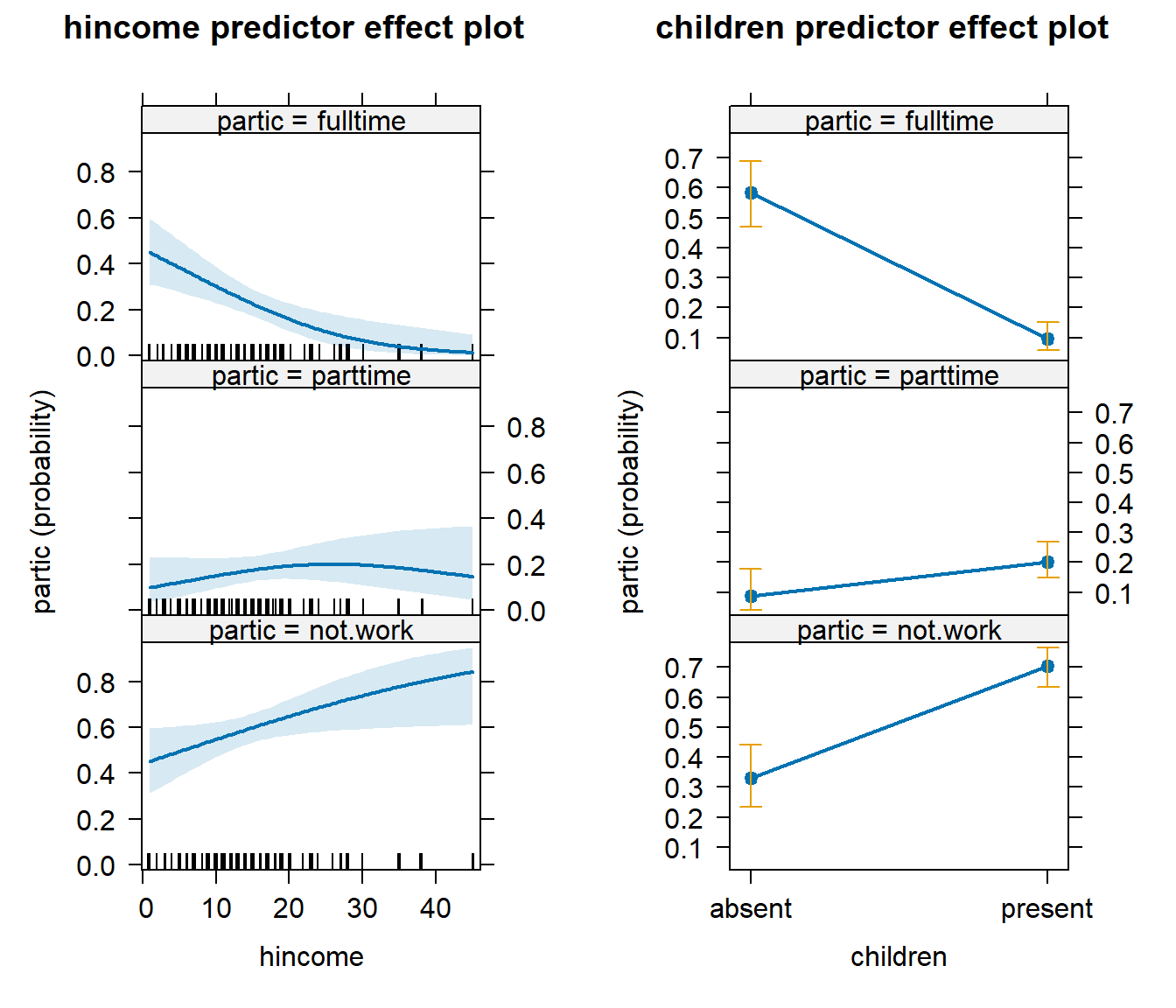

Default predictor effect plots for the nested-logit model fit to the Womenlf data

The panel at the left shows the predictor effect plot for husband’s income, that at the right the predictor effect plot for presence of children.

Because the model is additive, there are no conditioning variables in either plot. Effect plots are generally more interesting in models with interactions, in which case the effect plot for a predictor is conditioned on the other predictors with which the focal predictor interacts (see ?Effect.nestedLogit for an example).

In the predictor effect plot for hincome, the factor children is by default fixed to its distribution in the data; in the predictor effect plot for children, the numeric predictor hincome is by default fixed to its mean. The band in the graph at the left and vertical bars in the graph at the right give 95% confidence limits around the fit.

An alternative style of effect plot shows the fit as a stacked-area graph (in this case without confidence limits):

plot(predictorEffects(wlf.nested),
     axes=list(y=list(style="stacked")),
     lines=list(col=scales::hue_pal()(3)))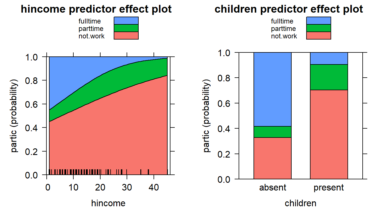

Stacked-area predictor effect plots for the nested-logit model fit to the Womenlf data

The computation and display of effect graphs are highly customizable. For details, see the documentation for the effects package.

Effect plots for nestedLogit models are also supported in the ggeffects package (Lüdecke, 2023). For example, the following (not run) produces plots of predicted probabilities for the same model with separate panels for the levels of partic.

ggpredict(wlf.nested, c("hincome[all]", "children")) |> plot()

Alternative models for the Womenlf data

We’ve mentioned that the nested dichotomies {not working} vs. {part-time, full-time} and {part-time} vs. {full-time} for the Womenlf data are largely arbitrary. An alternative set of nested dichotomies first contrasts full-time work with the other categories, {full-time} vs. {not working, part-time}, and then {not working} vs. {part-time}. The rationale is that the real hurdle for young married women to enter the paid labor force is to combine full-time work outside the home with housework. This alternative nested-dichotomies model proves enlightening:

wlf.nested.alt <- nestedLogit(partic ~ hincome + children,
                              logits(full=dichotomy(nonfulltime=c("not.work", "parttime"), "fulltime"),
                                     part=dichotomy("not.work", "parttime")),
                              data=Womenlf)

The Anova() and summary() for this model show that the effects of husband’s income and children make a substantial contribution to the full model but not to the part model:

Anova(wlf.nested.alt)
#> 
#>  Analysis of Deviance Tables (Type II tests)
#>  
#> Response full: nonfulltime{not.work, parttime} vs. {fulltime}
#>          LR Chisq Df Pr(>Chisq)    
#> hincome      15.1  1      1e-04 ***
#> children     63.6  1    1.6e-15 ***
#> ---
#> Signif. codes:  0 '***' 0.001 '**' 0.01 '*' 0.05 '.' 0.1 ' ' 1
#> 
#> 
#> Response part: {not.work} vs. {parttime}
#>          LR Chisq Df Pr(>Chisq)
#> hincome    0.0851  1       0.77
#> children   0.0012  1       0.97
#> 
#> 
#> Combined Responses
#>          LR Chisq Df Pr(>Chisq)    
#> hincome      15.2  2    0.00051 ***
#> children     63.6  2    1.6e-14 ***
#> ---
#> Signif. codes:  0 '***' 0.001 '**' 0.01 '*' 0.05 '.' 0.1 ' ' 1

summary(wlf.nested.alt)
#> Nested logit models: partic ~ hincome + children
#> 
#> Response full: nonfulltime{not.work, parttime} vs. {fulltime}
#> Call:
#> glm(formula = full ~ hincome + children, family = binomial, data = Womenlf, 
#>     contrasts = contrasts)
#> 
#> Deviance Residuals: 
#>    Min      1Q  Median      3Q     Max  
#> -1.745  -0.583  -0.443   0.242   2.378  
#> 
#> Coefficients:
#>                 Estimate Std. Error z value Pr(>|z|)    
#> (Intercept)       1.7696     0.4690    3.77  0.00016 ***
#> hincome          -0.0987     0.0277   -3.57  0.00036 ***
#> childrenpresent  -2.5631     0.3489   -7.35    2e-13 ***
#> ---
#> Signif. codes:  0 '***' 0.001 '**' 0.01 '*' 0.05 '.' 0.1 ' ' 1
#> 
#> (Dispersion parameter for binomial family taken to be 1)
#> 
#>     Null deviance: 296.34  on 262  degrees of freedom
#> Residual deviance: 218.81  on 260  degrees of freedom
#> AIC: 224.8
#> 
#> Number of Fisher Scoring iterations: 5
#> 
#> Response part: {not.work} vs. {parttime}
#> Call:
#> glm(formula = part ~ hincome + children, family = binomial, data = Womenlf, 
#>     contrasts = contrasts)
#> 
#> Deviance Residuals: 
#>    Min      1Q  Median      3Q     Max  
#> -0.757  -0.696  -0.688  -0.671   1.794  
#> 
#> Coefficients:
#>                 Estimate Std. Error z value Pr(>|z|)  
#> (Intercept)     -1.42758    0.58222   -2.45    0.014 *
#> hincome          0.00687    0.02343    0.29    0.769  
#> childrenpresent  0.01629    0.46762    0.03    0.972  
#> ---
#> Signif. codes:  0 '***' 0.001 '**' 0.01 '*' 0.05 '.' 0.1 ' ' 1
#> 
#> (Dispersion parameter for binomial family taken to be 1)
#> 
#>     Null deviance: 204.16  on 196  degrees of freedom
#> Residual deviance: 204.07  on 194  degrees of freedom
#>   (66 observations deleted due to missingness)
#> AIC: 210.1
#> 
#> Number of Fisher Scoring iterations: 4

It’s apparent that the alternative model produces a simpler description of the data: The predictors husband’s income and presence of children affect the decision to work full-time, but not the decision to work part-time among those who aren’t engaged in full-time work.

But do the fits of the two models to the data differ? We can compare fitted probabilities under the two specifications:

fit1 <- predict(wlf.nested)$p
fit2 <- predict(wlf.nested.alt)$p
diag(cor(fit1, fit2))
#> not.work parttime fulltime 
#>   0.9801   0.9185   0.9961
mean(as.matrix(abs(fit1 - fit2)))
#> [1] 0.01712
max(abs(fit1 - fit2))
#> [1] 0.1484

The fitted probabilities are similar but far from the same.

The two models have the same number of parameters and neither is nested within the other, so a conventional likelihood-ratio test is inappropriate, but we can still compare maximized log-likelihoods under the two models:

logLik(wlf.nested)
#> 'log Lik.' -212.1 (df=6)
logLik(wlf.nested.alt)
#> 'log Lik.' -211.4 (df=6)

Because the sample sizes and numbers of parameters are the same for the two models, differences in AIC and BIC are just twice the differences in the log-likelihoods; for example:

AIC(wlf.nested, wlf.nested.alt)
#>                df   AIC
#> wlf.nested      6 436.2
#> wlf.nested.alt  6 434.9

The comparison slightly favors the alternative nested-dichotomies model.

Here’s a graph of the alternative model:

op <- par(mfcol=c(1, 2), mar=c(4, 4, 3, 1) + 0.1)
col <- scales::hue_pal()(3)
plot(wlf.nested.alt, "hincome",           # left panel
     others = list(children="absent"), 
     xlab="Husband's Income", 
     legend.location="top", col = col)
plot(wlf.nested.alt, "hincome",           # right panel
     others = list(children="present"),
     xlab="Husband's Income", 
     legend=FALSE, col = col)
par(op)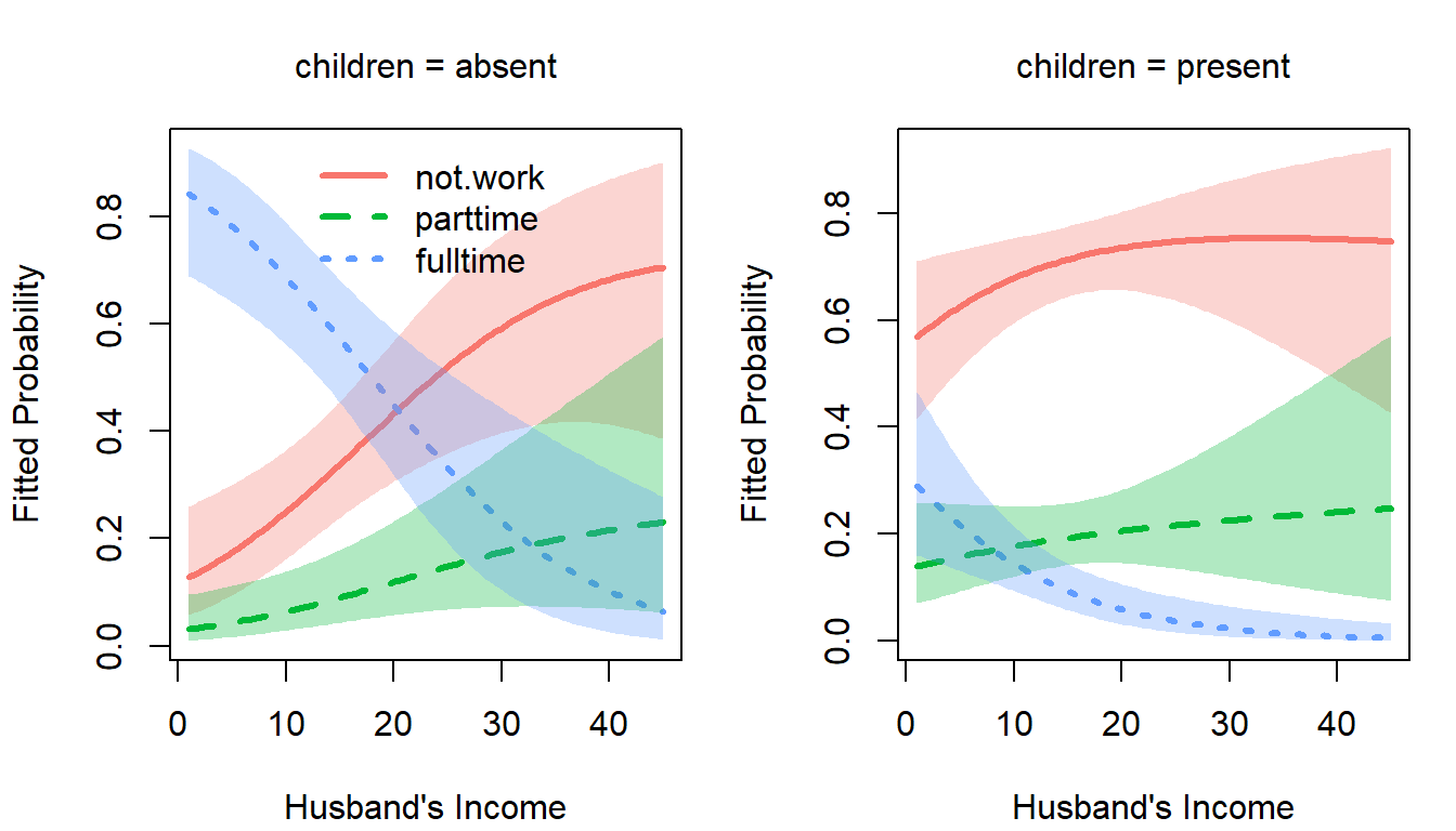

Predicted probabilities for the alternative nested-dichotomies model

Compare this to the previous graph for the original specification.

It’s also of interest to compare the nested-dichotomies models to the multinomial logit model, which, as we explained, treats the response categories symmetrically:

wlf.multinom <- multinom(partic ~ hincome + children, data = Womenlf)
#> # weights:  12 (6 variable)
#> initial  value 288.935032 
#> iter  10 value 211.454772
#> final  value 211.440963 
#> converged
summary(wlf.multinom)
#> Call:
#> multinom(formula = partic ~ hincome + children, data = Womenlf)
#> 
#> Coefficients:
#>          (Intercept)   hincome childrenpresent
#> parttime      -1.432  0.006894         0.02146
#> fulltime       1.983 -0.097232        -2.55861
#> 
#> Std. Errors:
#>          (Intercept) hincome childrenpresent
#> parttime      0.5925 0.02345          0.4690
#> fulltime      0.4842 0.02810          0.3622
#> 
#> Residual Deviance: 422.9 
#> AIC: 434.9
logLik(wlf.multinom)
#> 'log Lik.' -211.4 (df=6)

Check the relationship between fitted probabilities:

fit3 <- predict(wlf.multinom, type="probs")[, c("not.work", "parttime", "fulltime")]
diag(cor(fit2, fit3))
#> not.work parttime fulltime 
#>        1        1        1
mean(as.matrix(abs(fit2 - fit3)))
#> [1] 0.0001251
max(abs(fit2 - fit3))
#> [1] 0.0006908

As it turns out, the multinomial logit model and the alternative nested-dichotomies model produce nearly identical fits with similar simple interpretations.

References

Anderson, D., Heiss, A., & Sumners, J. (2023). Equatiomatic: Transform models into LaTeX equations.

Atkinson, T., Blishen, B. R., Ornstein, M. D., & Stevenson, H. M. (1984). Quality of Canadian Life: Social Change in Canada, 1977. ICPSR - Interuniversity Consortium for Political; Social Research. http://doi.org/10.3886/ICPSR07879.V1

Fienberg, S. E. (1980). The analysis of cross-classified categorical data (Second edition). Cambridge, MA: MIT Press.

Fox, J. (1984). Linear statistical models and related methods. New York: Wiley.

Fox, J. (2003). Effect displays in R for generalised linear models. Journal of Statistical Software, 8(15), 1–27. http://doi.org/10.18637/jss.v008.i15

Fox, J. (2016). Applied regression analysis and generalized linear models (Third edition). Thousand Oaks CA: SAGE. Retrieved from https://www.john-fox.ca/AppliedRegression/index.html

Fox, J., & Hong, J. (2009). Effect displays in R for multinomial and proportional-odds logit models: Extensions to the effects package. Journal of Statistical Software, 32(1), 1–24. http://doi.org/10.18637/jss.v032.i01

Fox, J., & Weisberg, S. (2018). Visualizing fit and lack of fit in complex regression models with predictor effect plots and partial residuals. Journal of Statistical Software, 87(9), 1–27. http://doi.org/10.18637/jss.v087.i09

Fox, J., & Weisberg, S. (2019). An R companion to applied regression (Third edition). Thousand Oaks CA: Sage. Retrieved from https://www.john-fox.ca/Companion/index.html

Fox, J., Weisberg, S., & Price, B. (2022). carData: Companion to applied regression data sets. Retrieved from https://CRAN.R-project.org/package=carData

Fox, J., Weisberg, S., & Price, B. (2023). Car: Companion to applied regression. Retrieved from https://CRAN.R-project.org/package=car

Friendly, M., & Meyer, D. (2016). Discrete data analysis with R: Visualization and modeling techniques for categorical and count data. Boca Raton, FL: Chapman & Hall/CRC.

Lüdecke, D. (2023). Ggeffects: Create tidy data frames of marginal effects for ggplot from model outputs. Retrieved from https://strengejacke.github.io/ggeffects/

Robinson, D., Hayes, A., & Couch, S. (2023). Broom: Convert statistical objects into tidy tibbles. Retrieved from https://CRAN.R-project.org/package=broom

Venables, W. N., & Ripley, B. D. (2002). Modern applied statistics with s (Fourth). New York: Springer. Retrieved from https://www.stats.ox.ac.uk/pub/MASS4/