Extract Binary Logit Models from a nestedLogit Object

Nested logit models represent an overall models for a polytomous response (>2 categories) by a set of binary logit models corresponding to nested dichotomies among the response categories. models is used to extract "glm" objects representing binary logit models from a "nestedLogit" object.

Usage

models(model, select, as.list = FALSE)

# S3 method for class 'nestedLogit'
models(model, select, as.list = FALSE)

Arguments

model

a "nestedLogit" model.

select

a numeric or character vector giving the number(s) or names(s) of one or more binary logit models to be extracted from model; if absent, a list of all of the binary logits models in model is returned.

as.list

if TRUE (the default is FALSE) and one binary logit model is selected, return the "glm" object in a one-element named list; otherwise a single model is returned directly as a "glm" object; when more than one binary logit model is selected, the corresponding "glm" objects are always returned as a named list.

Value

model returns either a single "glm" object (see glm) or a list of "glm" objects, each representing a binary logit model.

Examples

  data("Womenlf", package = "carData")
  comparisons <- logits(work=dichotomy("not.work",
                                       working=c("parttime", "fulltime")),
                        full=dichotomy("parttime", "fulltime"))
  m <- nestedLogit(partic ~ hincome + children,
                   dichotomies = comparisons,
                   data=Womenlf)

  # extract both submodels, as a list
  models(m, c("work", "full"))
#> $work
#> 
#> Call:  glm(formula = work ~ hincome + children, family = binomial, data = Womenlf, 
#>     contrasts = contrasts)
#> 
#> Coefficients:
#>     (Intercept)          hincome  childrenpresent  
#>         1.33583         -0.04231         -1.57565  
#> 
#> Degrees of Freedom: 262 Total (i.e. Null);  260 Residual
#> Null Deviance:	    356.2 
#> Residual Deviance: 319.7 	AIC: 325.7
#> 
#> $full
#> 
#> Call:  glm(formula = full ~ hincome + children, family = binomial, data = Womenlf, 
#>     contrasts = contrasts)
#> 
#> Coefficients:
#>     (Intercept)          hincome  childrenpresent  
#>          3.4778          -0.1073          -2.6515  
#> 
#> Degrees of Freedom: 107 Total (i.e. Null);  105 Residual
#>   (155 observations deleted due to missingness)
#> Null Deviance:	    144.3 
#> Residual Deviance: 104.5 	AIC: 110.5
#> 

  # extract the binomial logit model for working vs. non-working
  m_work <- models(m, "work")

  # use that to plot residuals
  plot(density(residuals(m_work)))


  # or plot that model -- gives the 'regression quartet' for a glm()
  op <- par(mfrow = c(2,2))
  plot(m_work)

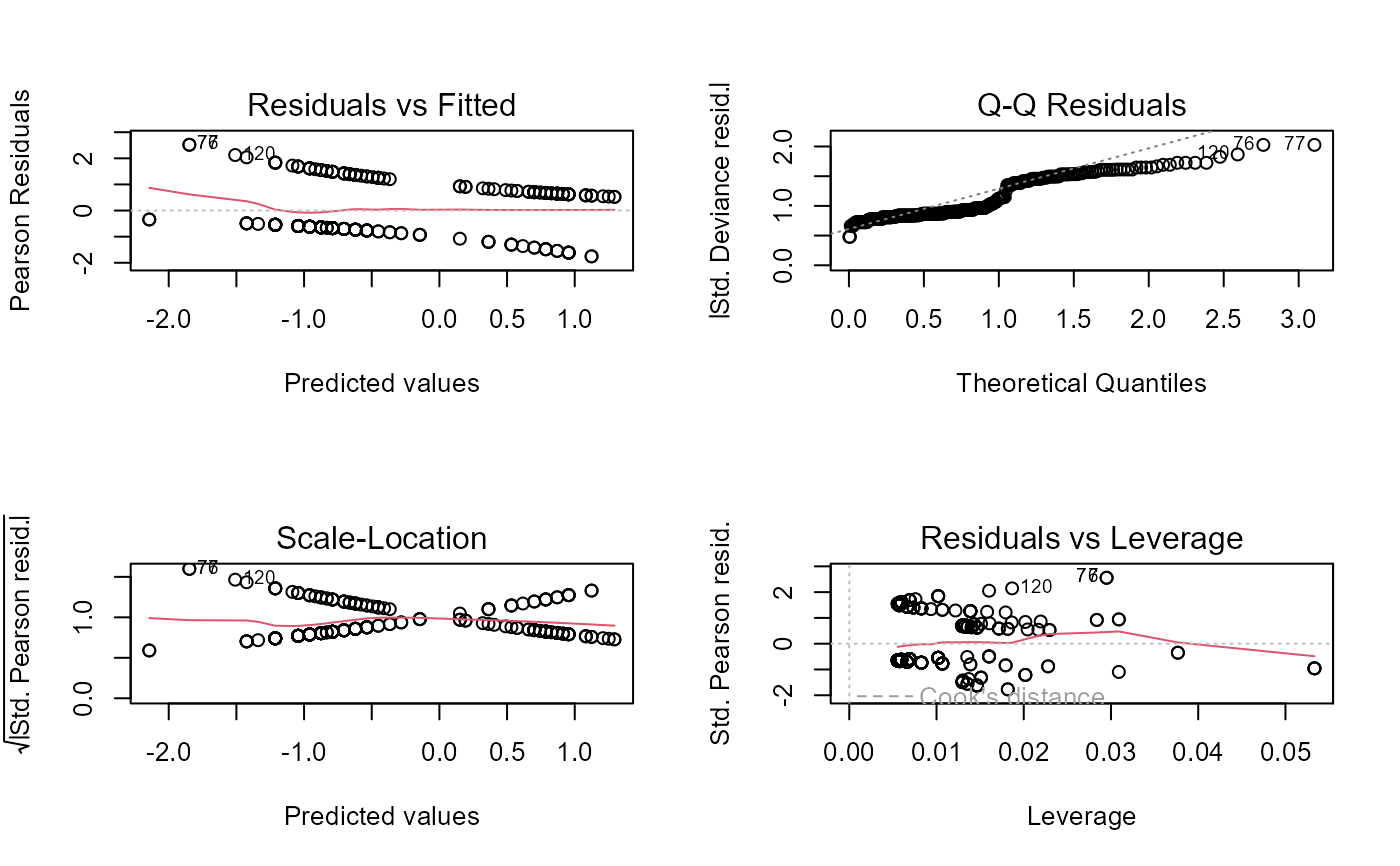  par(op)