This data set is drawn from the U.S. General Social Survey (GSS) for years between 1972 and 2016.
Usage
data("GSS", package = "nestedLogit")Format
A data frame with 44091 rows and 3 columns.
- parentdeg
A factor representing parents' attained level of education (highest "degree" obtained), recording the higher of mother's and father's education, with levels
"<highschool","highschool","college", and"graduate".- degree
The respondent's level of education, a factor with the same levels as
parentdeg.- year
The year of the survey, between
1972and2016.
Source
General Social Survey, NORC, The University of Chicago https://www.norc.org/Research/Projects/Pages/general-social-survey.aspx.
Examples
round(100*with(GSS, prop.table(table(degree, parentdeg), 2)))
#> parentdeg
#> degree <highschool highschool college graduate
#> <highschool 39 8 2 2
#> highschool 51 68 47 35
#> college 6 17 36 36
#> graduate 4 7 15 27
m.GSS <- nestedLogit(degree ~ parentdeg*year,
continuationLogits(c("<highschool", "highschool",
"college", "graduate")),
data=GSS)
car::Anova(m.GSS)
#>
#> Analysis of Deviance Tables (Type II tests)
#>
#> Response above_.highschool: {<highschool} vs. {highschool, college, graduate}
#> LR Chisq Df Pr(>Chisq)
#> parentdeg 6604.2 3 <2e-16 ***
#> year 383.3 1 <2e-16 ***
#> parentdeg:year 3.4 3 0.3297
#> ---
#> Signif. codes: 0 '***' 0.001 '**' 0.01 '*' 0.05 '.' 0.1 ' ' 1
#>
#>
#> Response above_highschool: {highschool} vs. {college, graduate}
#> LR Chisq Df Pr(>Chisq)
#> parentdeg 3541.7 3 <2e-16 ***
#> year 159.8 1 <2e-16 ***
#> parentdeg:year 1.6 3 0.6597
#> ---
#> Signif. codes: 0 '***' 0.001 '**' 0.01 '*' 0.05 '.' 0.1 ' ' 1
#>
#>
#> Response above_college: {college} vs. {graduate}
#> LR Chisq Df Pr(>Chisq)
#> parentdeg 121.317 3 < 2.2e-16 ***
#> year 29.074 1 6.966e-08 ***
#> parentdeg:year 3.294 3 0.3485
#> ---
#> Signif. codes: 0 '***' 0.001 '**' 0.01 '*' 0.05 '.' 0.1 ' ' 1
#>
#>
#> Combined Responses
#> LR Chisq Df Pr(>Chisq)
#> parentdeg 10267.2 9 <2e-16 ***
#> year 572.1 3 <2e-16 ***
#> parentdeg:year 8.3 9 0.5018
#> ---
#> Signif. codes: 0 '***' 0.001 '**' 0.01 '*' 0.05 '.' 0.1 ' ' 1
summary(m.GSS)
#> Nested logit models: degree ~ parentdeg * year
#> <environment: 0x000001754fe79940>
#>
#> Response above_.highschool: {<highschool} vs. {highschool, college, graduate}
#> Call:
#> glm(formula = above_.highschool ~ parentdeg * year, family = binomial,
#> data = GSS, contrasts = contrasts)
#>
#> Coefficients:
#> Estimate Std. Error z value Pr(>|z|)
#> (Intercept) -4.177e+01 2.692e+00 -15.519 <2e-16 ***
#> parentdeghighschool 6.388e-01 4.971e+00 0.129 0.8977
#> parentdegcollege 2.167e+00 1.499e+01 0.145 0.8851
#> parentdeggraduate -3.443e+01 2.051e+01 -1.679 0.0931 .
#> year 2.121e-02 1.353e-03 15.675 <2e-16 ***
#> parentdeghighschool:year 6.655e-04 2.496e-03 0.267 0.7898
#> parentdegcollege:year 4.694e-04 7.515e-03 0.062 0.9502
#> parentdeggraduate:year 1.895e-02 1.029e-02 1.841 0.0656 .
#> ---
#> Signif. codes: 0 '***' 0.001 '**' 0.01 '*' 0.05 '.' 0.1 ' ' 1
#>
#> (Dispersion parameter for binomial family taken to be 1)
#>
#> Null deviance: 40989 on 44090 degrees of freedom
#> Residual deviance: 32877 on 44083 degrees of freedom
#> AIC: 32893
#>
#> Number of Fisher Scoring iterations: 6
#>
#> Response above_highschool: {highschool} vs. {college, graduate}
#> Call:
#> glm(formula = above_highschool ~ parentdeg * year, family = binomial,
#> data = GSS, contrasts = contrasts)
#>
#> Coefficients:
#> Estimate Std. Error z value Pr(>|z|)
#> (Intercept) -2.605e+01 4.468e+00 -5.829 5.56e-09 ***
#> parentdeghighschool 9.091e-01 5.196e+00 0.175 0.861
#> parentdegcollege 4.089e+00 6.542e+00 0.625 0.532
#> parentdeggraduate -4.807e+00 7.527e+00 -0.639 0.523
#> year 1.223e-02 2.243e-03 5.454 4.93e-08 ***
#> parentdeghighschool:year -1.542e-04 2.607e-03 -0.059 0.953
#> parentdegcollege:year -1.193e-03 3.279e-03 -0.364 0.716
#> parentdeggraduate:year 3.513e-03 3.772e-03 0.931 0.352
#> ---
#> Signif. codes: 0 '***' 0.001 '**' 0.01 '*' 0.05 '.' 0.1 ' ' 1
#>
#> (Dispersion parameter for binomial family taken to be 1)
#>
#> Null deviance: 44729 on 36343 degrees of freedom
#> Residual deviance: 40691 on 36336 degrees of freedom
#> (7747 observations deleted due to missingness)
#> AIC: 40707
#>
#> Number of Fisher Scoring iterations: 4
#>
#> Response above_college: {college} vs. {graduate}
#> Call:
#> glm(formula = above_college ~ parentdeg * year, family = binomial,
#> data = GSS, contrasts = contrasts)
#>
#> Coefficients:
#> Estimate Std. Error z value Pr(>|z|)
#> (Intercept) -5.591941 8.422569 -0.664 0.5067
#> parentdeghighschool -15.751212 9.787684 -1.609 0.1076
#> parentdegcollege -18.936884 11.182715 -1.693 0.0904 .
#> parentdeggraduate -10.230758 11.213329 -0.912 0.3616
#> year 0.002556 0.004226 0.605 0.5453
#> parentdeghighschool:year 0.007727 0.004909 1.574 0.1154
#> parentdegcollege:year 0.009285 0.005604 1.657 0.0975 .
#> parentdeggraduate:year 0.005210 0.005619 0.927 0.3538
#> ---
#> Signif. codes: 0 '***' 0.001 '**' 0.01 '*' 0.05 '.' 0.1 ' ' 1
#>
#> (Dispersion parameter for binomial family taken to be 1)
#>
#> Null deviance: 14195 on 11098 degrees of freedom
#> Residual deviance: 14042 on 11091 degrees of freedom
#> (32992 observations deleted due to missingness)
#> AIC: 14058
#>
#> Number of Fisher Scoring iterations: 4
#>
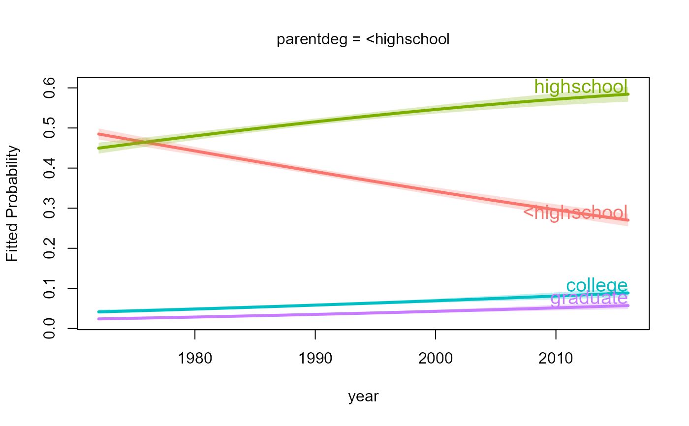
# plot fitted probabilities
plot(m.GSS, x.var = "year",
others = list(parentdeg = "<highschool"),
lty = 1,
label = TRUE)
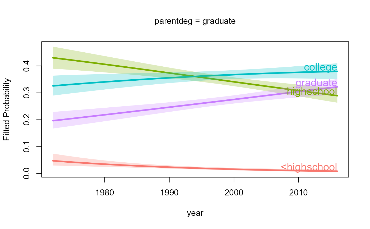
 plot(m.GSS, x.var = "year",
others = list(parentdeg = "graduate"),
lty = 1,
label = TRUE)
plot(m.GSS, x.var = "year",
others = list(parentdeg = "graduate"),
lty = 1,
label = TRUE)