A plot method for "nestedLogit" objects produced by the
nestedLogit function. Fitted probabilities under the model,
or the corresponding logits are plotted
for each level of the polytomous response variable, with one of the explanatory variables
on the horizontal axis and other explanatory variables fixed to particular values.
By default, a 95% pointwise confidence envelope is added to the plot.
Usage
# S3 method for class 'nestedLogit'
plot(
  x,
  x.var,
  others,
  n.x.values = 100L,
  scale = c("prob", "logit"),
  xlab = x.var,
  ylab = NULL,
  main,
  cex.main = 1,
  digits.main = getOption("digits") - 2L,
  font.main = 1L,
  pch = 1L:length(response.levels),
  lwd = 3,
  lty = 1L:length(response.levels),
  col = (scales::hue_pal())(length(response.levels)),
  legend = TRUE,
  legend.inset = 0.01,
  legend.location = "topleft",
  legend.bty = "n",
  conf.level = 0.95,
  conf.alpha = 0.25,
  label = FALSE,
  label.x = "max",
  label.cex = 1.25,
  label.col = col,
  ...
)
Arguments
- x
an object of
"nestedLogit"produced bynestedLogit.- x.var
quoted name of the variable to appear on the x-axis; if omitted, the first predictor in the model is used.
- others
a named list of values for the other variables in the model, that is, other than
x.var; if any other predictor is omitted, it is set to an arbitrary value—the mean for a numeric predictor or the first level or value of a factor, character, or logical predictor; only one value may be specified for each variable inothers.- n.x.values
the number of evenly spaced values of
x.varat which to evaluate fitted probabilities to be plotted (default100).- scale
character string;
"prob"(the default) plots fitted probabilities on the y-axis;"logit"plots fitted log odds (logits), i.e., \(\log(p/(1-p))\).- xlab
label for the x-axis (defaults to the value of
x.var).- ylab
label for the y-axis (defaults to
"Fitted Probability"whenscale = "prob"and"Fitted Log Odds"whenscale = "logit").- main
main title for the graph (if missing, constructed from the variables and values in
others).- cex.main
size of main title (see
par).- digits.main
number of digits to retain when rounding values for the main title.
- font.main
font for main title (see
par).- pch
plotting characters (see
par).- lwd
line width (see
par).- lty
line types (see
par).- col
line colors for the response levels (see
par).- legend
if
TRUE(the default), add a legend for the response levels to the graph. Ignored whenlabel = TRUE.- legend.inset
default
0.01(seelegend).- legend.location
position of the legend (default
"topleft", seelegend).- legend.bty
the type of box to be drawn around the legend. The allowed values are "o" (the default) and "n".
- conf.level
the level for pointwise confidence envelopes around the predicted values; the default is
0.95. IfNULL, the confidence envelopes are suppressed.- conf.alpha
the opacity of the confidence envelopes; the default is
0.3.- label
if
TRUE, label the curves directly instead of using a legend. Default isFALSE.- label.x
where to place the label for each curve. Either a single string,
"min"or"max"(applied to all curves), or a character vector of length equal to the number of response categories with each element being"min"or"max", e.g.label.x = c("min", "max", "max")."min"places the label at the left end of the curve;"max"(the default) places it at the right end.- label.cex
character expansion factor for direct labels; default
1.25.- label.col
colors for direct labels; defaults to
col, so labels match their curves. Supply a vector of length equal to the number of response categories to use different colors for the labels.- ...
arguments to be passed to
matplot.
Examples
data("Womenlf", package = "carData")
m <- nestedLogit(partic ~ hincome + children,
logits(work=dichotomy("not.work", c("parttime", "fulltime")),
full=dichotomy("parttime", "fulltime")),
data=Womenlf)
plot(m, legend.location="top")
#> Note: hincome will be used for the horizontal axis
#> Note: missing predictor children set to its first level, 'absent'
 op <- par(mfcol=c(1, 2), mar=c(4, 4, 3, 1) + 0.1)
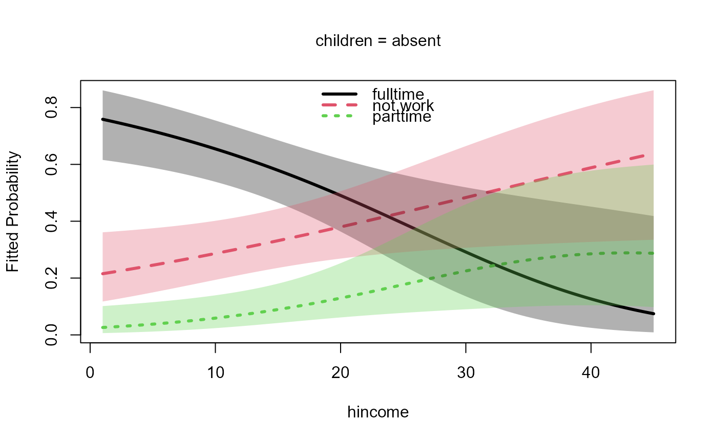
plot(m, "hincome", list(children="absent"),
xlab="Husband's Income", legend=FALSE)
plot(m, "hincome", list(children="present"),
xlab="Husband's Income")
op <- par(mfcol=c(1, 2), mar=c(4, 4, 3, 1) + 0.1)
plot(m, "hincome", list(children="absent"),
xlab="Husband's Income", legend=FALSE)
plot(m, "hincome", list(children="present"),
xlab="Husband's Income")
 par(op)
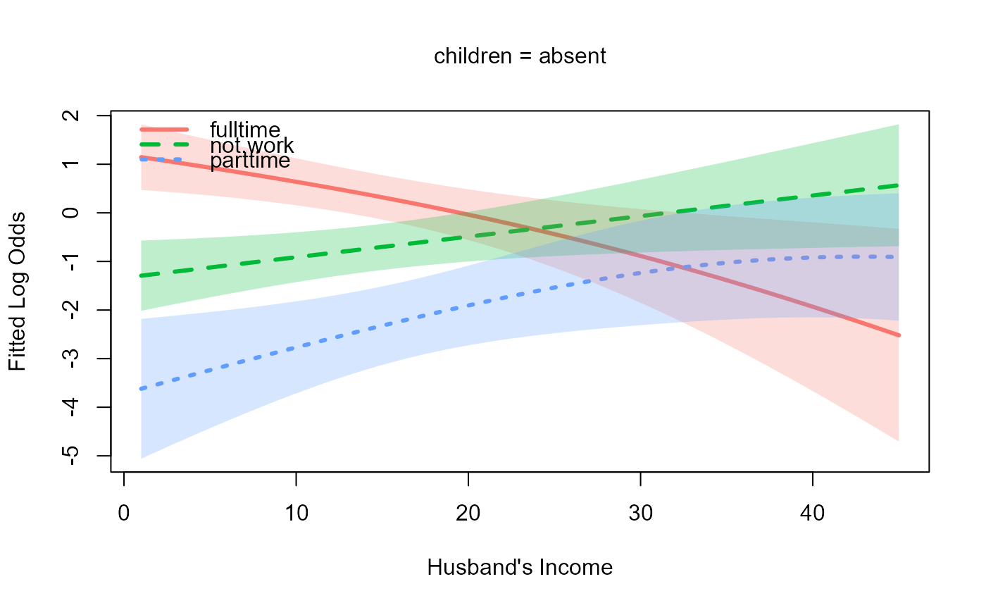
# Plot on the logit (log-odds) scale
plot(m, "hincome", list(children="absent"), scale = "logit",
xlab = "Husband's Income")
par(op)
# Plot on the logit (log-odds) scale
plot(m, "hincome", list(children="absent"), scale = "logit",
xlab = "Husband's Income")
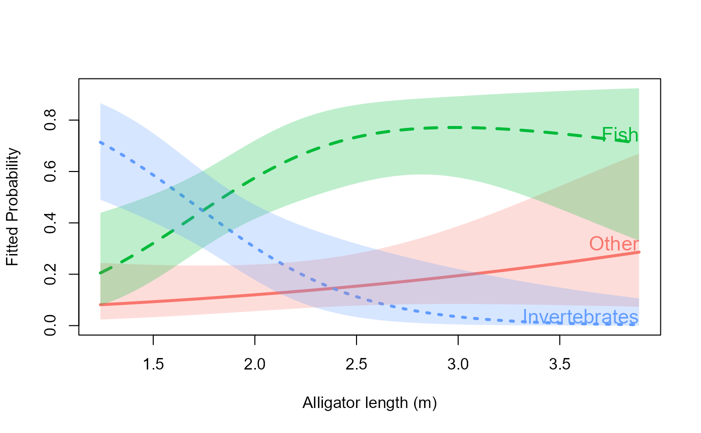
 # Gators example: direct curve labels instead of a legend
data("gators", package = "nestedLogit")
gators.nested <- nestedLogit(food ~ length,
logits(d1 = dichotomy("Other", c("Fish", "Invertebrates")),
d2 = dichotomy("Fish", "Invertebrates")),
data = gators)
# All labels at the right end (default)
plot(gators.nested, x.var = "length", label = TRUE,
xlab = "Alligator length (m)")
# Gators example: direct curve labels instead of a legend
data("gators", package = "nestedLogit")
gators.nested <- nestedLogit(food ~ length,
logits(d1 = dichotomy("Other", c("Fish", "Invertebrates")),
d2 = dichotomy("Fish", "Invertebrates")),
data = gators)
# All labels at the right end (default)
plot(gators.nested, x.var = "length", label = TRUE,
xlab = "Alligator length (m)")
 # Mixed placement: Other and Invertebrates labeled at left, Fish at right
# (food levels are: "Other", "Fish", "Invertebrates")
plot(gators.nested, x.var = "length", label = TRUE,
label.x = c("min", "max", "min"),
xlab = "Alligator length (m)")
# Mixed placement: Other and Invertebrates labeled at left, Fish at right
# (food levels are: "Other", "Fish", "Invertebrates")
plot(gators.nested, x.var = "length", label = TRUE,
label.x = c("min", "max", "min"),
xlab = "Alligator length (m)")
