1a. Steps Toward Tidy Categorical Data Analysis

Overview

While R provides many intuitive facilities for the manipulation of continuous variables (such as those in the tidyverse collection of packages), it somewhat lacks the equivalent for categorical data. Two such areas include the collapsing of variable levels (e.g., combining hair colours of “Brown” and “Black” into a “Dark” category) and the conversion between forms of categorical data (e.g., from a table of entries to a data.frame containing frequencies for each combination of variable levels).

Tidy Collapsing

In R, when trying to collapse levels of a variable in a dataset (e.g., combining hair colours of “Brown” and “Black” into a “Dark” category), it was often the case that one would need to first convert amongst forms, “collapse” their data, aggregate the duplicate rows, and finally convert back to the initial form.

collapse_levels() simplifies this process, allowing for the intuitive collapsing of variable levels for datasets of any form. One just needs to ensure that an argument of freq = "the frequency column name" is supplied when the inputted dataset is in frequency form.

Functionality of collapse_levels() is demonstrated below using the starwars data from the dplyr package. This dataset contains case form data on various characters in the Star Wars franchise. Variables considered in this vignette are a character’s hair_color, skin_color, and eye_color. Taken as is, this would correspond to an \(11 \times 28 \times 15\) contingency table… Time to collapse!

Here I load the starwars data and select the variables of interest. For simplicity, I then remove rows containing NA values.

data("starwars", package = "dplyr")

star_case <- starwars |>
  dplyr::select(c("hair_color", "skin_color", "eye_color")) |> 
  tidyr::drop_na()

str(star_case)
## tibble [82 × 3] (S3: tbl_df/tbl/data.frame)
##  $ hair_color: chr [1:82] "blond" "none" "brown" "brown, grey" ...
##  $ skin_color: chr [1:82] "fair" "white" "light" "light" ...
##  $ eye_color : chr [1:82] "blue" "yellow" "brown" "blue" ...

First, taking a look at the levels of variable hair_color, there are many ways one might want to collapse these categories:

unique(star_case$hair_color)
##  [1] "blond"         "none"          "brown"         "brown, grey"  
##  [5] "black"         "auburn, white" "auburn, grey"  "white"        
##  [9] "grey"          "auburn"        "blonde"

Example: Likely the most natural of these ways is the following:

Collapse different spellings of "blond" (i.e., "blond" and "blonde" become Blonde).
Collapse different shades of "brown" (i.e., "brown" and "brown, grey" become Brown).
Collapse different shades of "auburn" (i.e., "auburn, white", "auburn, grey", and "auburn" become Auburn).
Keep "none" as-is.
Keep "white" as-is.
Keep "grey" as-is.
Keep "Black" as-is.

Here is how to do this using collapse_levels():

collapsed.star_case <- collapse_levels(
  star_case,             # The dataset
  hair_color = list(     # Assign the variable to be collapsed to a list
    
    # Format the list as NewLevel = c("old1", "old2", ..., "oldn")
    Blonde = c("blond", "blonde"), 
    Brown = c("brown", "brown, grey"),
    Auburn = c("auburn, white", "auburn, grey", "auburn")
  )
)
str(collapsed.star_case)
## tibble [82 × 3] (S3: tbl_df/tbl/data.frame)
##  $ hair_color: Factor w/ 7 levels "Auburn","black",..: 3 6 4 4 4 2 1 3 1 4 ...
##  $ skin_color: chr [1:82] "fair" "white" "light" "light" ...
##  $ eye_color : chr [1:82] "blue" "yellow" "brown" "blue" ...
unique(collapsed.star_case$hair_color)
## [1] Blonde none   Brown  black  Auburn white  grey  
## Levels: Auburn black Blonde Brown grey none white

Second, one might also want to collapse levels of variable skin_color:

unique(star_case$skin_color)
##  [1] "fair"                "white"               "light"              
##  [4] "unknown"             "green"               "pale"               
##  [7] "metal"               "dark"                "brown mottle"       
## [10] "brown"               "grey"                "mottled green"      
## [13] "orange"              "blue, grey"          "grey, red"          
## [16] "red"                 "blue"                "grey, blue"         
## [19] "white, blue"         "grey, green, yellow" "yellow"             
## [22] "tan"                 "fair, green, yellow" "silver, red"        
## [25] "green, grey"         "red, blue, white"    "brown, white"       
## [28] "none"

Example: I decided to arbitrarily collapse these as follows:

Keep "none" as-is.
Keep"unknown" as-is.
Shades, comprising all levels that begin with "white", "grey", "dark", "light", and "fair".
Rainbows, comprising all other levels.

Note that when working with real data, arbitrary decisions involving the collapsing of variable levels are a VERY bad idea. Collapses should be grounded in strong, data-driven justification. Arbitrary collapsing is employed in this vignette purely for pedagogical and illustrative purposes.

collapsed.star_case <- collapse_levels(
  collapsed.star_case,
  skin_color = list(
    Shades = c(
      "fair", "white", "light", "dark", "grey", "grey, red", 
      "grey, blue", "white, blue", "grey, green, yellow", "fair, green, yellow"
    ), 
    Rainbows = c(
      "green", "pale", "metal", "brown mottle", "brown", "mottled green", 
      "orange", "blue, grey", "red", "blue", "yellow", "tan", "silver, red",
      "green, grey", "red, blue, white", "brown, white"
    )
  )
)
str(collapsed.star_case)
## tibble [82 × 3] (S3: tbl_df/tbl/data.frame)
##  $ hair_color: Factor w/ 7 levels "Auburn","black",..: 3 6 4 4 4 2 1 3 1 4 ...
##  $ skin_color: Factor w/ 4 levels "Rainbows","Shades",..: 2 2 2 2 2 2 2 2 2 4 ...
##  $ eye_color : chr [1:82] "blue" "yellow" "brown" "blue" ...
unique(collapsed.star_case$skin_color)
## [1] Shades   unknown  Rainbows none    
## Levels: Rainbows Shades none unknown

Third, one may also want to collapse levels of variable eye_color:

unique(star_case$eye_color)
##  [1] "blue"          "yellow"        "brown"         "blue-gray"    
##  [5] "hazel"         "red"           "orange"        "black"        
##  [9] "pink"          "unknown"       "red, blue"     "gold"         
## [13] "green, yellow" "white"         "dark"

Example: Again, I decided to arbitrarily collapse these as follows:

Normal, with levels of typical human eye color (i.e., "blue", "blue-gray", "brown", "hazel", and "dark").
Abnormal, with levels of eye colours that would be abnormal for humans (e.g., "red", "pink", "gold", etc.).
Keep unknown as-is.

collapsed.star_case <- collapse_levels(
  collapsed.star_case,
  eye_color = list(
    Normal = c("blue", "brown", "blue-gray", "hazel", "dark"), 
    Abnormal = c(
      "yellow", "red", "orange", "black", "pink", "red, blue", "gold", 
      "green, yellow", "white"
    )
  )
)
str(collapsed.star_case)
## tibble [82 × 3] (S3: tbl_df/tbl/data.frame)
##  $ hair_color: Factor w/ 7 levels "Auburn","black",..: 3 6 4 4 4 2 1 3 1 4 ...
##  $ skin_color: Factor w/ 4 levels "Rainbows","Shades",..: 2 2 2 2 2 2 2 2 2 4 ...
##  $ eye_color : Factor w/ 3 levels "Abnormal","Normal",..: 2 1 2 2 2 2 2 2 2 2 ...
unique(collapsed.star_case$eye_color)
## [1] Normal   Abnormal unknown 
## Levels: Abnormal Normal unknown

In addition, one may want (and is able) to collapse levels of multiple variables in a single call to collapse_levels().

Example: To illustrate this (and to provide an easy working example for the following “Tidy Conversions” section), the collapsed.star_case data is arbitrarily collapsed as follows to correspond to a \(3 \times 3 \times 3\) contingency table:

Variable hair_color:
1. Dark corresponding to levels "Brown", "black", and "Auburn".
2. Light corresponding to levels "Blonde", "white", and "grey".
3. Keep "none" as-is.
Variable skin_color:
1. Other corresponding to levels "none" and "unknown".
2. Keep Rainbows as-is.
3. Keep Shades as-is.
Variable eye_color kept as-is.

collapsed.star_case <- collapse_levels(
  collapsed.star_case,
  hair_color = list(    # First variable
    Dark = c("Brown", "black", "Auburn"),
    Light = c("Blonde", "white", "grey")
  ),
  skin_color = list(    # Second variable
    Other = c("none", "unknown")
  )
)
unique(collapsed.star_case$hair_color)
## [1] Light none  Dark 
## Levels: Dark Light none
unique(collapsed.star_case$skin_color)
## [1] Shades   Other    Rainbows
## Levels: Rainbows Shades Other
str(collapsed.star_case)
## tibble [82 × 3] (S3: tbl_df/tbl/data.frame)
##  $ hair_color: Factor w/ 3 levels "Dark","Light",..: 2 3 1 1 1 1 1 2 1 1 ...
##  $ skin_color: Factor w/ 3 levels "Rainbows","Shades",..: 2 2 2 2 2 2 2 2 2 3 ...
##  $ eye_color : Factor w/ 3 levels "Abnormal","Normal",..: 2 1 2 2 2 2 2 2 2 2 ...

Tidy Conversions

Until now, converting amongst forms of categorical data in R has been somewhat onerous. As outlined in 1. Creating and manipulating frequency tables, the below table shows the typical process for converting among forms (A, B, and C represent categorical variables, X represents an R data object):

From this		To this
	Case form	Frequency form	Table form
Case form	noop	`xtabs(~A+B)`	`table(A,B)`
Frequency form	`expand.dft(X)`	noop	`xtabs(count~A+B)`
Table form	`expand.dft(X)`	`as.data.frame(X)`	noop

Instead, one may simply use as_table(X) to convert to table form, as_freqform(X) to convert to frequency form, and as_caseform(X) to convert to case form. These are illustrated in the network (node/edge) diagram below:

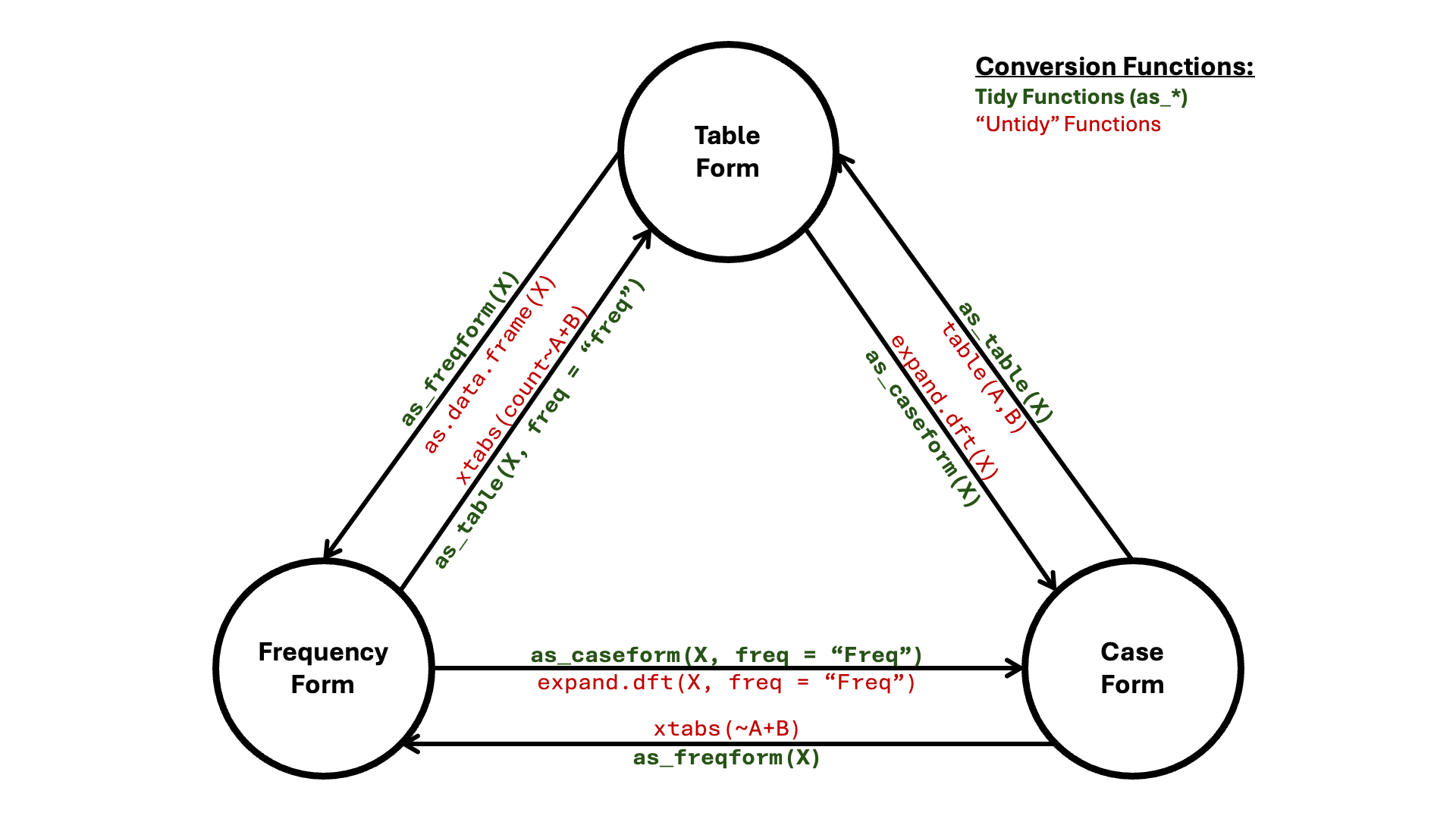
Additionally, there are functions as_array(X) and as_matrix(X) for converting to those respective types.

Like collapse_levels(), the single thing to keep in mind when employing these functions is the following: when your object X is in frequency form, an argument of freq = "your frequency column name" must be supplied. Besides this, the rote memory work of having to remember which function to use to convert form X to form Y is now completely removed.

Functionality of these “tidy” conversion functions are demonstrated below using the collapsed.star_case data from the most recent example (i.e., the data corresponding to a \(3 \times 3 \times 3\) contingency table).

Example: Convert the collapsed.star_case data into frequency form. Name this data star_freqform.

star_freqform <- as_freqform(collapsed.star_case)

str(star_freqform)
## tibble [27 × 4] (S3: tbl_df/tbl/data.frame)
##  $ hair_color: Factor w/ 3 levels "Dark","Light",..: 1 2 3 1 2 3 1 2 3 1 ...
##  $ skin_color: Factor w/ 3 levels "Rainbows","Shades",..: 1 1 1 2 2 2 3 3 3 1 ...
##  $ eye_color : Factor w/ 3 levels "Abnormal","Normal",..: 1 1 1 1 1 1 1 1 1 2 ...
##  $ Freq      : int [1:27] 1 2 18 0 1 11 0 0 1 7 ...

Note that if one would like a data frame instead of a tibble, an argument of tidy = FALSE needs to be provided. Naturally, this tidy argument is present only in functions as_freqform() and as_caseform().

Example: Convert the collapsed.star_case data into a data frame in frequency form.

as_freqform(collapsed.star_case, tidy = FALSE) |> str()
## 'data.frame':    27 obs. of  4 variables:
##  $ hair_color: Factor w/ 3 levels "Dark","Light",..: 1 2 3 1 2 3 1 2 3 1 ...
##  $ skin_color: Factor w/ 3 levels "Rainbows","Shades",..: 1 1 1 2 2 2 3 3 3 1 ...
##  $ eye_color : Factor w/ 3 levels "Abnormal","Normal",..: 1 1 1 1 1 1 1 1 1 2 ...
##  $ Freq      : int  1 2 18 0 1 11 0 0 1 7 ...

Example: Convert the frequency form data, star_freqform, into table form. Name this data star_tab. Because we are converting from frequency form, the freq = "frequency column name" argument must be supplied.

star_tab <- as_table(star_freqform, freq = "Freq")

str(star_tab)
##  'xtabs' int [1:3, 1:3, 1:3] 1 2 18 0 1 11 0 0 1 7 ...
##  - attr(*, "dimnames")=List of 3
##   ..$ hair_color: chr [1:3] "Dark" "Light" "none"
##   ..$ skin_color: chr [1:3] "Rainbows" "Shades" "Other"
##   ..$ eye_color : chr [1:3] "Abnormal" "Normal" "unknown"
##  - attr(*, "call")= language xtabs(formula = reformulate(cols, response = freq), data = obj)

Example: Convert the table form data, star_tab, into an array. Name this data star_array.

star_array <- as_array(star_tab)

class(star_array)
## [1] "array"
str(star_array)
##  int [1:3, 1:3, 1:3] 1 2 18 0 1 11 0 0 1 7 ...
##  - attr(*, "dimnames")=List of 3
##   ..$ hair_color: chr [1:3] "Dark" "Light" "none"
##   ..$ skin_color: chr [1:3] "Rainbows" "Shades" "Other"
##   ..$ eye_color : chr [1:3] "Abnormal" "Normal" "unknown"
##  - attr(*, "call")= language xtabs(formula = reformulate(cols, response = freq), data = obj)

To convert to a matrix, one also needs to specify row and column dimensions. This is done using the dims = c("dim1", "dim2", ..., "dim_n") argument, which works by summing over the dimensions excluded from this call. The first provided dimension is taken as the row dimension, with the second dimension taken as the column dimension.

Example: Convert the array form data, star_array, into a matrix with dimensions "hair_color" and "eye_color". Name this data star_mat.

star_mat <- as_matrix(star_array, dims = c("hair_color", "eye_color"))

class(star_mat)
## [1] "matrix" "array"
str(star_mat)
##  int [1:3, 1:3] 1 3 30 34 6 5 0 0 3
##  - attr(*, "dimnames")=List of 2
##   ..$ hair_color: chr [1:3] "Dark" "Light" "none"
##   ..$ eye_color : chr [1:3] "Abnormal" "Normal" "unknown"

Note that the dims argument works the same way for all other tidy conversion functions.

Example: Convert the table form data, star_tab, into frequency form with dimensions "hair_color" and "eye_color".

as_freqform(star_tab, dims = c("hair_color", "eye_color")) |> str()
## tibble [9 × 3] (S3: tbl_df/tbl/data.frame)
##  $ hair_color: Factor w/ 3 levels "Dark","Light",..: 1 2 3 1 2 3 1 2 3
##  $ eye_color : Factor w/ 3 levels "Abnormal","Normal",..: 1 1 1 2 2 2 3 3 3
##  $ Freq      : int [1:9] 1 3 30 34 6 5 0 0 3

Proportions

The last piece of these conversion functions is the prop argument, allowing users to convert cells/frequencies to proportions. Calculated proportions may either be relative to the grand total (prop = TRUE) or to one or more margins (prop = c("margin1", "margin2", ... "margin_n")).

Note that as_caseform() is the only of the tidy conversion functions to not include a prop argument. Also, as_caseform() will not convert proportional data.¹

Example: Convert star_mat into a table of proportions that are relative to the grand total.

star_mat # To view the original
##           eye_color
## hair_color Abnormal Normal unknown
##      Dark         1     34       0
##      Light        3      6       0
##      none        30      5       3

as_table(star_mat, prop = TRUE)
##           eye_color
## hair_color   Abnormal     Normal    unknown
##      Dark  0.01219512 0.41463415 0.00000000
##      Light 0.03658537 0.07317073 0.00000000
##      none  0.36585366 0.06097561 0.03658537

Example: Convert star_mat into a table of proportions that are relative to the marginal sums of hair_color.

as_table(star_mat, prop = "hair_color")
##           eye_color
## hair_color   Abnormal     Normal    unknown
##      Dark  0.02857143 0.97142857 0.00000000
##      Light 0.33333333 0.66666667 0.00000000
##      none  0.78947368 0.13157895 0.07894737

Example: Convert star_mat into a table of proportions that are relative to the marginal sums of both hair_color and eye_color. Since these are the only two dimensions, cell proportions will all be equal to \(1.0\) (except for cells where no data exists).

as_table(star_mat, prop = c("hair_color", "eye_color"))
##           eye_color
## hair_color Abnormal Normal unknown
##      Dark         1      1        
##      Light        1      1        
##      none         1      1       1

Taken Together

Taking collapse_levels() and the tidy conversion functions together, one now has an intuitive framework for manipulating categorical data.

Example: The starwars data also has a variable named homeworld, specifying the planet that a given character was from. The below code does the following:

Create data home_star from dataset starwars. The new data includes both homeworld and the previous variables of interest (hair_color, eye_color, and skin_color). Missing values are then omitted.
Sort homeworld alphabetically.
Collapse the first half of the sorted homeworlds into a level named abc.
Collapse the second half of the sorted homeworlds into a level named xyz.
Collapse eye_color according to the previous Abnormal, Normal, and "unknown" conventions.
Convert the collapsed data into a table with dimensions homeworld and eye_color. Call this table tab.home_star and plot the result in a mosaic display.
Convert tab.home_star into a matrix of proportions (relative to the grand total).

home_star <- starwars |>
  dplyr::select(c("hair_color", "skin_color", "eye_color", "homeworld")) |> 
  tidyr::drop_na()

# Sort unique levels of homeworld
lvls <- home_star$homeworld |> unique() |> sort()
lvls
##  [1] "Alderaan"       "Aleen Minor"    "Bespin"         "Bestine IV"    
##  [5] "Cato Neimoidia" "Cerea"          "Champala"       "Chandrila"     
##  [9] "Concord Dawn"   "Corellia"       "Coruscant"      "Dathomir"      
## [13] "Dorin"          "Endor"          "Eriadu"         "Geonosis"      
## [17] "Glee Anselm"    "Haruun Kal"     "Iktotch"        "Iridonia"      
## [21] "Kalee"          "Kamino"         "Kashyyyk"       "Malastare"     
## [25] "Mirial"         "Mon Cala"       "Muunilinst"     "Naboo"         
## [29] "Ojom"           "Quermia"        "Ryloth"         "Serenno"       
## [33] "Shili"          "Skako"          "Socorro"        "Stewjon"       
## [37] "Sullust"        "Tatooine"       "Toydaria"       "Trandosha"     
## [41] "Troiken"        "Tund"           "Umbara"         "Utapau"        
## [45] "Vulpter"        "Zolan"

# Collapse variable levels
collapsed.home_star <- collapse_levels(
  home_star,
  homeworld = list(
    abc = lvls[1:(length(lvls)/2)],
    xyz = lvls[(length(lvls)/2 + 1):length(lvls)]
  ),
  eye_color = list(
    Normal = c("blue", "brown", "blue-gray", "hazel", "dark"), 
    Abnormal = c(
      "yellow", "red", "orange", "black", "pink", "red, blue", "gold", 
      "green, yellow", "white"
    )
  )
)
# Convert to table of dimensions 'homeworld' and 'eye_color'
tab.home_star <- as_table(collapsed.home_star, dims = c("homeworld", "eye_color"))

# Plot as mosaic display
mosaic(tab.home_star, shading = TRUE, gp = shading_Friendly)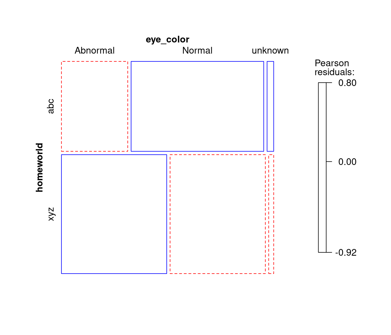


# Convert table into matrix of proportions. Note argument 'dims' was not supplied
# as we already know that there are exactly 2 dimensions.
as_matrix(tab.home_star, prop = TRUE)
##          eye_color
## homeworld  Abnormal    Normal    unknown
##       abc 0.1388889 0.2777778 0.01388889
##       xyz 0.2916667 0.2638889 0.01388889
## attr(,"call")
## xtabs(formula = reformulate(cols), data = obj)

Thus, this constitutes a pipeline for working with categorical data:

Gather data and clean it.
Collapse levels when substantively necessary.
Convert forms, select dimensions, and/or take proportions if necessary.

dataset |>                             # Gather the data
  select(...) |> drop_na() |> ... |>   # Clean the data
  collapse_levels(...) |>              # Collapse levels as necessary
  as_form(...)   # Convert forms, select dimensions, take proportions

When viewed this way, these functions appear to be the start of a grammar of categorical data analysis.

May the Forms Be with You: Novel Functions to Intuitively Convert Among Forms and Collapse Variable Levels Presented Using the `starwars` Data.

Gavin M. Klorfine

Overview

Tidy Collapsing

Tidy Conversions

Proportions

Taken Together

1a. Steps Toward Tidy Categorical Data Analysis

May the Forms Be with You: Novel Functions to Intuitively Convert Among Forms and Collapse Variable Levels Presented Using the starwars Data.

Gavin M. Klorfine

Overview

Tidy Collapsing

Tidy Conversions

Proportions

Taken Together

May the Forms Be with You: Novel Functions to Intuitively Convert Among Forms and Collapse Variable Levels Presented Using the `starwars` Data.