Extensions and additions to vcd: Visualizing Categorical Data
Version 0.9.6; documentation built for pkgdown 2026-06-05
This package provides additional data sets, documentation, and many functions designed to extend the vcd package for Visualizing Categorical Data and the gnm package for Generalized Nonlinear Models. In particular, vcdExtra extends mosaic, assoc and sieve plots from vcd to handle glm() and gnm() models and adds a 3D version in mosaic3d().
The functions here use the “strucplot” framework (Meyer et-al., 2006), which is a lovely, natural conceptual system for implementing visualization and other displays for n-way frequency tables which have a nested, hierarchical structure in vcd. [This can be compared to the “productplots” framework in producplots, and the defunct ggmosaic package]
vcdExtra also adds extensions to modeling functions for models fit using glm() and MASS::loglm(), using the construct glmlist() to construct a list of related models which can be summarized (via LRstats()) and graphed (via mosaic.glmlist())
vcdExtra is a support package for the book Discrete Data Analysis with R (DDAR) by Michael Friendly and David Meyer. There is also a web site for DDAR with all figures and code samples from the book. It is also used in my graduate course, Psy 6136: Categorical Data Analysis.
A more general goal of vcdExtra is to contribute to the wider topics of thinking about, analyzing and visualizing categorical data, extending this beyond the scope of our book. In this sense, it continues to be a love letter 💌 to CDA.
📂 Installation
Get the released version (0.9.3) from CRAN:
The current development version (0.9.6) can be installed from R-universe or directly from the GitHub repo via:
 if (!require(remotes)) install.packages("remotes")
 install.packages("vcdExtra", repos = c('https://friendly.r-universe.dev')
 # or
 remotes::install_github("friendly/vcdExtra", build_vignettes = TRUE)
Overview
The original purpose of this package was to serve as a sandbox for introducing extensions of mosaic plots and related graphical methods that apply to loglinear models fitted using MASS::loglm(), generalized linear models using stats::glm() and the related, generalized nonlinear models fitted with gnm() in the gnm package.
A related purpose was to fill in some holes in the analysis of categorical data in R, not provided in base R, vcd, or other commonly used packages.
See also:
![]()
![]()
My book, Discrete Data Analysis with R: Visualization and Modeling Techniques for Categorical and Count Data
My graduate course, Psy 6136: Categorical Data Analysis
A companion package,
nestedLogit, for fitting nested dichotomy logistic regression models for a polytomous response.
💡 vcdExtra Highlights
What’s in the box?
Mosaic plot extensions
The method
mosaic.glm()extends themosaic.loglm()method in the vcd package to this wider class of models, e.g., models for ordinal factors, which can’t be handled withMASS::loglm(). This method also works for the generalized nonlinear models fit with the gnm package, including models for square tables and models with multiplicative associations (RC models).mosaic3d()introduces a 3D generalization of mosaic displays using the rgl package.A new “labeling” method,
labeling_points()for mosaic plots allows you to show the observed or expected frequencies in cells as point symbols, thereby showing the data or model in a dot-density representation. This goes back to an old paper, Friendly(1995), where I describe visual and conceptual models for categorical data with a physical analog of gas molecules in chambers.
Model extensions
A new class,
glmlist, is introduced for working with collections of glm objects, e.g.,Kway()for fitting all K-way models from a basic marginal model, andLRstats()for brief statistical summaries of goodness-of-fit for a collection of models.Similarly, for loglinear models fit using
MASS::loglm(), the functionseq_loglm()fits a series of sequential models to the 1-, 2-, … n-way marginal tables, corresponding to a variety of types of models for joint, conditional, mutual, … independence. It returns an object of classloglmlist, each of which is a classloglmobject. The functionseq_mosaic()generates the mosaic plots and other plots in thevcd::strucplot()framework.For square tables with ordered factors,
Crossings()supplements the specification of terms in model formulas usinggnm::Symm(),gnm::Diag(),gnm::Topo(),etc. in the gnm package.
🗃️ Datasets
Beyond the wide range of **datasets* in the vcd package, this vcdExtra package includes many new data sets, that I’ve found useful for illustrating various ideas, models, methods and visualization. Use datasets("vcdExtra") to see a list with titles and descriptions. The vignette, vignette("datasets", package="vcdExtra") provides a classification of these according to methods of analysis.
vcdExtra::datasets("vcdExtra")[,1]
##  [1] "Abortion"       "Accident"       "AirCrash"       "Alligator"
##  [5] "Asbestos"       "Bartlett"       "Burt"           "Caesar"
##  [9] "Cancer"         "Cormorants"     "CrabSatellites" "CyclingDeaths"
## [13] "DaytonSurvey"   "Depends"        "Detergent"      "Donner"
## [17] "Draft1970"      "Draft1970table" "Dyke"           "Fungicide"
## [21] "GSS"            "Geissler"       "Gilby"          "Glass"
## [25] "HairEyePlace"   "Hauser79"       "Heart"          "Heckman"
## [29] "HospVisits"     "HouseTasks"     "Hoyt"           "ICU"
## [33] "JobSat"         "Mammograms"     "Mental"         "Mice"
## [37] "Mobility"       "PhdPubs"        "Reinis"         "ShakeWords"
## [41] "TV"             "Titanicp"       "Toxaemia"       "Vietnam"
## [45] "Vote1980"       "WorkerSat"      "Yamaguchi87"
📖 Vignettes
A collection of tutorial vignettes. In the installed package, they can be viewed using browseVignettes(package = "vcdExtra");
vigns <- as.data.frame(tools::getVignetteInfo("vcdExtra")[,c("File", "Title")])
vigns$Title <- paste0("[", vigns$Title, "](https://friendly.github.io/vcdExtra/articles/",
                      tools::file_path_sans_ext(vigns$File), ".html)")
vigns |> knitr::kable()| File | Title |
|---|---|
| a1-creating.Rmd | 1. Creating and manipulating frequency tables |
| a1a-convert-collapse.Rmd | 1a. Steps Toward Tidy Categorical Data Analysis |
| a2-tests.Rmd | 2. Tests of Independence |
| a3-loglinear.Rmd | 3. Loglinear Models |
| a4-mosaics.Rmd | 4. Mosaic plots |
| a5-demo-housing.Rmd | 5. Demo - Housing Data |
| a6-mobility.Rmd | 6. Mobility tables |
| a7-continuous.Rmd | 7. Continuous predictors |
| datasets.Rmd | Datasets for categorical data analysis |
| tidyCats.Rmd | tidyCat: Tidy Methods For Categorical Data Analysis |
there is also a set of simple demonstration files illustrating analysis of datasets with more detail than provided in their individual help files. Use
demo(package = "vcdExtra")to see the list and rundemo("occStatus") to run the analysis for this example, ordemo(“mental-glm”)` for another one.a few useful utility functions for manipulating categorical data sets and working with models for categorical data:
joint(),conditional(),mutual(),saturated(). These make it easier to specifyloglm()andglm()models representing a statistical concept, like conditional association, rather than figuring out a formula like[AC] [BC]for a 3-way table or[AD] [BD] [CD]for a 4-way table.A re-implementation of
vcd::woolf_test()extends the analysis of homogeneity of odds ratios in 2 x 2 x R x C tables to provide tests for differences among the R strata rows and C strata columns.
Recent work
Visual tables
A new function, color_table() provides semi-graphic tables of frequency tables or residuals from a loglinear model. The essential idea is to use background shading of cells in the table to show patterns not discernible in purely numeric tables.
Association graphs
I’m now experimenting with using graphical association representations of models in conjunction with the other methods, and ways of specifying models here. assoc_graph() Association graphs represent variables as nodes and their partial associations between pairs of variables as edges. They are useful for understanding If two variables are not connected by an edge, they are conditionally independent given the other variables in the model.
How can we use this in practice, to understand a model, or how well it fits a given dataset?
There is now (rudimentary) a plot() method for association graphs which allows edges to be weighted by a measure of the strength of association between variables: partial \(G^2\) or Cramer’s V. Still very much a WIP.
📊 Examples
These README examples provide simple illustrations of using some of the package functions in the context of loglinear models for frequency tables fit using glm(), including models for structured associations taking ordinality into account.
Mental dataset
The dataset vcdExtra::Mental is a data frame frequency table representing the cross-classification of mental health status (mental) of 1660 young New York residents by their parents’ socioeconomic status (ses). Both are ordered factors. The questions are:
- Is
mentalhealth associated with parentsses? - If so, what is the pattern/nature of the association?
- How can I take the ordinal nature of the factors into account?
data(Mental)
str(Mental)
## 'data.frame':    24 obs. of  3 variables:
##  $ ses   : Ord.factor w/ 6 levels "1"<"2"<"3"<"4"<..: 1 1 1 1 2 2 2 2 3 3 ...
##  $ mental: Ord.factor w/ 4 levels "Well"<"Mild"<..: 1 2 3 4 1 2 3 4 1 2 ...
##  $ Freq  : int  64 94 58 46 57 94 54 40 57 105 ...

# show as frequency table
(Mental.tab <- xtabs(Freq ~ ses+mental, data=Mental))
##    mental
## ses Well Mild Moderate Impaired
##   1   64   94       58       46
##   2   57   94       54       40
##   3   57  105       65       60
##   4   72  141       77       94
##   5   36   97       54       78
##   6   21   71       54       71
Independence model
Fit the independence model, Freq ~ mental + ses, using glm(..., family = poisson) This model is equivalent to the chisq.test(Mental) for general association; it does not take ordinality into account. LRstats() provides a compact summary of fit statistics for one or more models.
indep <- glm(Freq ~ mental + ses,
             family = poisson, data = Mental)
LRstats(indep)
## Likelihood summary table:
##          AIC    BIC LR Chisq Df Pr(>Chisq)
## indep 209.59 220.19   47.418 15  3.155e-05 ***
## ---
## Signif. codes:  0 '***' 0.001 '**' 0.01 '*' 0.05 '.' 0.1 ' ' 1
mosaic.glm() is the mosaic method for glm objects. The default mosaic display for these data:
mosaic(indep)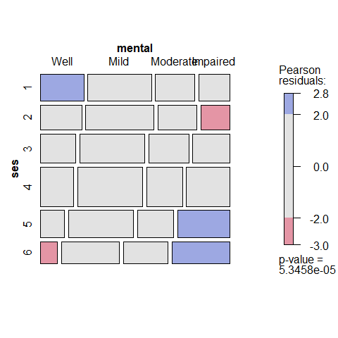
It is usually better to use standardized residuals (residuals_type="rstandard") in mosaic displays, rather than the default Pearson residuals. Here we also add longer labels for the table factors (set_varnames) and display the values of residuals (labeling=labeling_residuals) in the cells.
The strucplot formula argument, ~ ses + mental here gives the order of the factors in the mosaic display, not the statistical model for independence. That is, the unit square is first split by ses, then by mental within each level of ses.
# labels for table factors
long.labels <- list(set_varnames = c(mental="Mental Health Status",
                                     ses="Parent SES"))

mosaic(indep, formula = ~ ses + mental,
       residuals_type="rstandard",
       labeling_args = long.labels,
       labeling=labeling_residuals)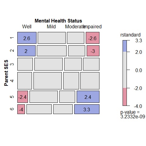
The opposite-corner pattern of the residuals clearly shows that association between Parent SES and mental health depends on the ordered levels of the factors: higher Parent SES is associated with better mental health status. A principal virtue of mosaic plots is to show the pattern of association that remains after a model has been fit, and thus help suggest a better model.
Ordinal models
Ordinal models use numeric scores for the row and/or column variables. These models typically use equally spaced integer scores. The test for association here is analogous to a test of the correlation between the frequency-weighted scores, carried out using CMHtest().
CMHtest(Mental.tab)
## Cochran-Mantel-Haenszel Statistics for ses by mental
##
##                  AltHypothesis  Chisq Df       Prob
## cor        Nonzero correlation 37.156  1 1.0907e-09
## rmeans  Row mean scores differ 40.297  5 1.3012e-07
## cmeans  Col mean scores differ 40.666  3 7.6971e-09
## general    General association 45.958 15 5.4003e-05
In the data, ses and mental were declared to be ordered factors, so using as.numeric(Mental$ses) is sufficient to create a new Cscore variable. Similarly for the numeric version of mental, giving Rscore.
Cscore <- as.numeric(Mental$ses)
Rscore <- as.numeric(Mental$mental)
Using these, the term Rscore:Cscore represents an association constrained to be linear x linear; that is, the slopes for profiles of mental health status are assumed to vary linearly with those for Parent SES. (This model asserts that only one parameter (a local odds ratio) is sufficient to account for all association, and is also called the model of “uniform association”.)
# fit linear x linear (uniform) association.  Use integer scores for rows/cols
Cscore <- as.numeric(Mental$ses)
Rscore <- as.numeric(Mental$mental)

linlin <- glm(Freq ~ mental + ses + Rscore:Cscore,
              family = poisson, data = Mental)
mosaic(linlin, ~ ses + mental,
       residuals_type="rstandard",
       labeling_args = long.labels,
       labeling=labeling_residuals,
       suppress=1,
       gp=shading_Friendly,
       main="Lin x Lin model")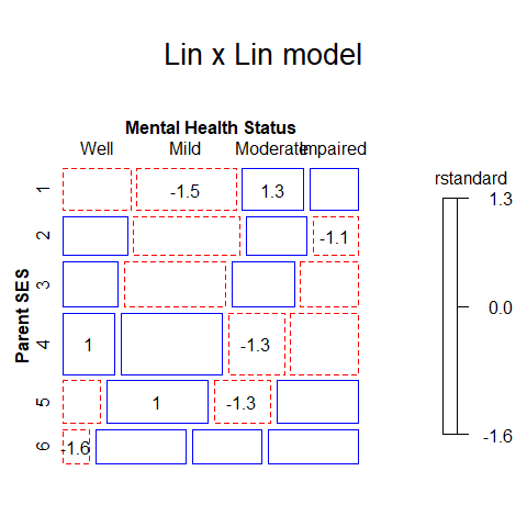
Note that the test for linear x linear association consumes only 1 degree of freedom, compared to the (r-1)*(c-1) = 15 degrees of freedom for general association.
anova(linlin, test="Chisq")
## Analysis of Deviance Table
##
## Model: poisson, link: log
##
## Response: Freq
##
## Terms added sequentially (first to last)
##
##
##               Df Deviance Resid. Df Resid. Dev  Pr(>Chi)
## NULL                             23    217.400
## mental         3  113.525        20    103.875 < 2.2e-16 ***
## ses            5   56.457        15     47.418 6.543e-11 ***
## Rscore:Cscore  1   37.523        14      9.895 9.035e-10 ***
## ---
## Signif. codes:  0 '***' 0.001 '**' 0.01 '*' 0.05 '.' 0.1 ' ' 1
Other models are possible between the independence model, Freq ~ mental + ses, and the saturated model Freq ~ mental + ses + mental:ses. The update.glm() method make these easy to specify, as addition of terms to the independence model.
# use update.glm method to fit other models

linlin <- update(indep, . ~ . + Rscore:Cscore)
roweff <- update(indep, . ~ . + mental:Cscore)
coleff <- update(indep, . ~ . + Rscore:ses)
rowcol <- update(indep, . ~ . + Rscore:ses + mental:Cscore)
Compare the models: For glm objects, the print and summary methods give too much information if all one wants to see is a brief summary of model goodness of fit, and there is no easy way to display a compact comparison of model goodness of fit for a collection of models fit to the same data.
LRstats() provides a brief summary for one or more models fit to the same dataset. The likelihood ratio \(\chi^2\) values (LR Chisq)test lack of fit. By these tests, none of the ordinal models show significant lack of fit. By the AIC and BIC statistics, the linlin model is the best, combining parsimony and goodness of fit.
LRstats(indep, linlin, roweff, coleff, rowcol)
## Likelihood summary table:
##           AIC    BIC LR Chisq Df Pr(>Chisq)
## indep  209.59 220.19   47.418 15  3.155e-05 ***
## linlin 174.07 185.85    9.895 14     0.7698
## roweff 174.45 188.59    6.281 12     0.9013
## coleff 179.00 195.50    6.829 10     0.7415
## rowcol 179.22 198.07    3.045  8     0.9315
## ---
## Signif. codes:  0 '***' 0.001 '**' 0.01 '*' 0.05 '.' 0.1 ' ' 1
The anova.glm() function gives tests of nested models.
anova(indep, linlin, roweff, test = "Chisq")
## Analysis of Deviance Table
##
## Model 1: Freq ~ mental + ses
## Model 2: Freq ~ mental + ses + Rscore:Cscore
## Model 3: Freq ~ mental + ses + mental:Cscore
##   Resid. Df Resid. Dev Df Deviance  Pr(>Chi)
## 1        15     47.418
## 2        14      9.895  1   37.523 9.035e-10 ***
## 3        12      6.281  2    3.614    0.1641
## ---
## Signif. codes:  0 '***' 0.001 '**' 0.01 '*' 0.05 '.' 0.1 ' ' 1
References
Friendly, M. (1995). Conceptual and Visual Models for Categorical Data. The American Statistician, 49, 153–160. http://www.datavis.ca/papers/amstat95.pdf
Friendly, M. & Meyer, D. (2016). Discrete Data Analysis with R: Visualization and Modeling Techniques for Categorical and Count Data. Boca Raton, FL: Chapman & Hall/CRC.
Meyer, D., Zeileis, A., & Hornik, K. (2006). The Strucplot Framework: Visualizing Multi-way Contingency Tables with vcd. Journal of Statistical Software, 17(3), 1–48. http://www.jstatsoft.org/v17/i03/