Mosaic plots for fitted generalized linear and generalized nonlinear models
Source:R/mosaic.glm.R
mosaic.glm.RdProduces mosaic plots (and other plots in the strucplot
framework) for a log-linear model fitted with glm or
for a generalized nonlinear model fitted with gnm.
Usage
# S3 method for class 'glm'
mosaic(
  x,
  formula = NULL,
  panel = mosaic,
  type = c("observed", "expected"),
  residuals = NULL,
  residuals_type = c("pearson", "deviance", "rstandard"),
  gp = shading_hcl,
  gp_args = list(),
  ...
)

# S3 method for class 'glm'
sieve(x, ...)

# S3 method for class 'glm'
assoc(x, ...)
Arguments
- x
A
glmorgnmobject. The response variable, typically a cell frequency, should be non-negative.- formula
A one-sided formula with the indexing factors of the plot separated by '+', determining the order in which the variables are used in the mosaic. A formula must be provided unless
x$datainherits from class"table"– in which case the indexing factors of this table are used, or the factors inx$data(or model.frame(x) ifx$datais an environment) exactly cross-classify the data – in which case this set of cross-classifying factors are used.- panel
Panel function used to draw the plot for visualizing the observed values, residuals and expected values. Currently, one of
"mosaic","assoc", or"sieve"invcd.- type
A character string indicating whether the
"observed"or the"expected"values of the table should be visualized by the area of the tiles or bars.- residuals
An optional array or vector of residuals corresponding to the cells in the data, for example, as calculated by
residuals.glm(x),residuals.gnm(x).- residuals_type
If the
residualsargument isNULL, residuals are calculated internally and used in the display. In this case,residual_typecan be"pearson","deviance"or"rstandard". Otherwise (whenresidualsis supplied),residuals_typeis used as a label for the legend in the plot.- gp
Object of class
"gpar", shading function or a corresponding generating function (seestrucplotDetails andshadings). Ignored if shade = FALSE.- gp_args
A list of arguments for the shading-generating function, if specified.
- ...
Other arguments passed to the
panelfunction e.g.,mosaic
Value
The structable visualized by strucplot is
returned invisibly.
Details
These methods extend the range of strucplot visualizations well beyond the
models that can be fit with loglm. They are intended for
models for counts using the Poisson family (or quasi-poisson), but should be
sensible as long as (a) the response variable is non-negative and (b) the
predictors visualized in the strucplot are discrete factors.
For both poisson family generalized linear models and loglinear models,
standardized residuals provided by rstandard (sometimes called
adjusted residuals) are often preferred because they have constant unit
asymptotic variance.
The sieve and assoc methods are simple convenience interfaces
to this plot method, setting the panel argument accordingly.
See also
glm, gnm,
plot.loglm, mosaic
Other mosaic plots:
mosaic.glmlist(),
mosaic3d()
Examples
library(vcdExtra)
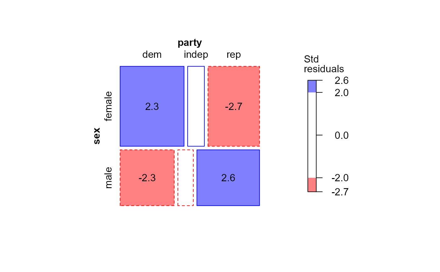
GSStab <- xtabs(count ~ sex + party, data=GSS)
# using the data in table form
mod.glm1 <- glm(Freq ~ sex + party, family = poisson, data = GSStab)
res <- residuals(mod.glm1)
std <- rstandard(mod.glm1)
# For mosaic.default(), need to re-shape residuals to conform to data
stdtab <- array(std,
dim=dim(GSStab),
dimnames=dimnames(GSStab))
mosaic(GSStab,
gp=shading_Friendly,
residuals=stdtab,
residuals_type="Std\nresiduals",
labeling = labeling_residuals)
 # Using externally calculated residuals with the glm() object
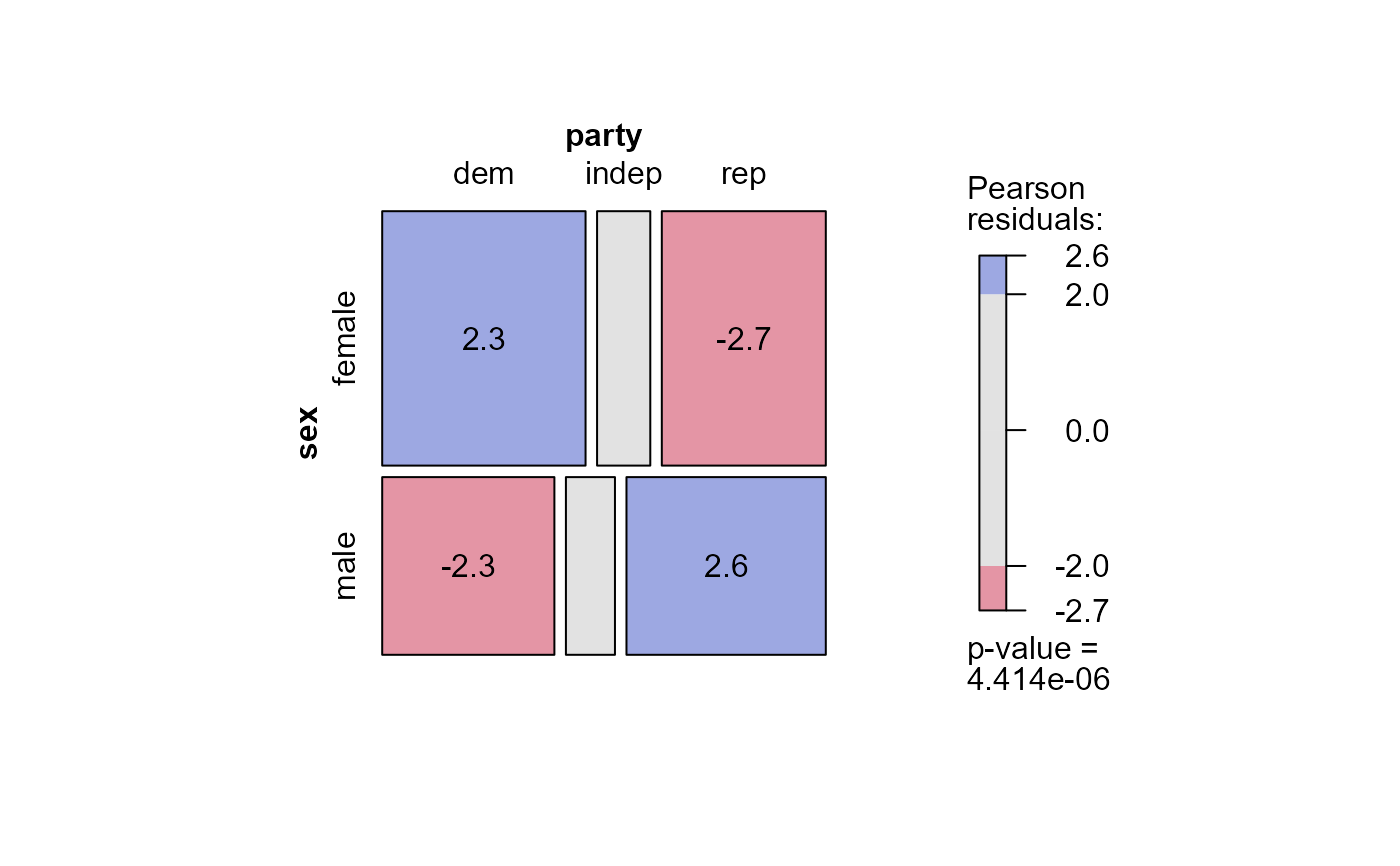
mosaic(mod.glm1,
residuals=std,
labeling = labeling_residuals,
shade=TRUE)
# Using externally calculated residuals with the glm() object
mosaic(mod.glm1,
residuals=std,
labeling = labeling_residuals,
shade=TRUE)
 # Using residuals_type
mosaic(mod.glm1,
residuals_type="rstandard",
labeling = labeling_residuals, shade=TRUE)
# Using residuals_type
mosaic(mod.glm1,
residuals_type="rstandard",
labeling = labeling_residuals, shade=TRUE)
 ## Ordinal factors and structured associations
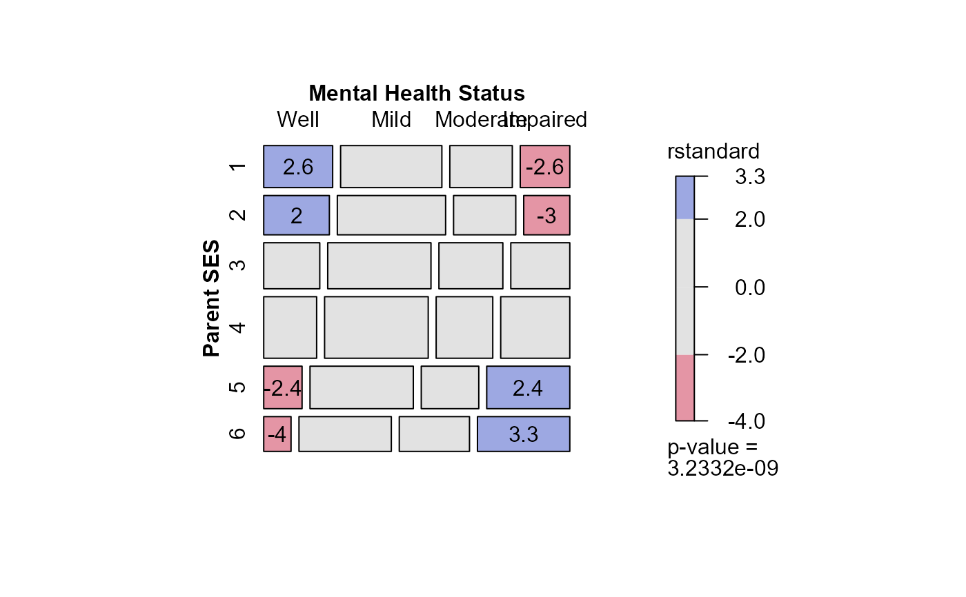
data(Mental)
xtabs(Freq ~ mental+ses, data=Mental)
#> ses
#> mental 1 2 3 4 5 6
#> Well 64 57 57 72 36 21
#> Mild 94 94 105 141 97 71
#> Moderate 58 54 65 77 54 54
#> Impaired 46 40 60 94 78 71
long.labels <- list(set_varnames = c(mental="Mental Health Status",
ses="Parent SES"))
# fit independence model
# Residual deviance: 47.418 on 15 degrees of freedom
indep <- glm(Freq ~ mental+ses,
family = poisson, data = Mental)
long.labels <- list(set_varnames = c(mental="Mental Health Status",
ses="Parent SES"))
mosaic(indep,
formula = ~ses + mental,
residuals_type="rstandard",
labeling_args = long.labels,
labeling=labeling_residuals)
## Ordinal factors and structured associations
data(Mental)
xtabs(Freq ~ mental+ses, data=Mental)
#> ses
#> mental 1 2 3 4 5 6
#> Well 64 57 57 72 36 21
#> Mild 94 94 105 141 97 71
#> Moderate 58 54 65 77 54 54
#> Impaired 46 40 60 94 78 71
long.labels <- list(set_varnames = c(mental="Mental Health Status",
ses="Parent SES"))
# fit independence model
# Residual deviance: 47.418 on 15 degrees of freedom
indep <- glm(Freq ~ mental+ses,
family = poisson, data = Mental)
long.labels <- list(set_varnames = c(mental="Mental Health Status",
ses="Parent SES"))
mosaic(indep,
formula = ~ses + mental,
residuals_type="rstandard",
labeling_args = long.labels,
labeling=labeling_residuals)
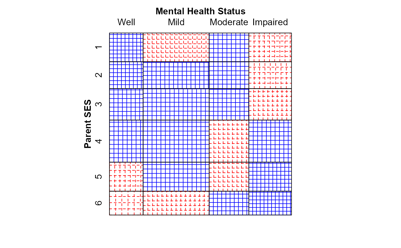
 # or, show as a sieve diagram
mosaic(indep,
formula = ~ses + mental,
labeling_args = long.labels,
panel=sieve,
gp=shading_Friendly)
# or, show as a sieve diagram
mosaic(indep,
formula = ~ses + mental,
labeling_args = long.labels,
panel=sieve,
gp=shading_Friendly)
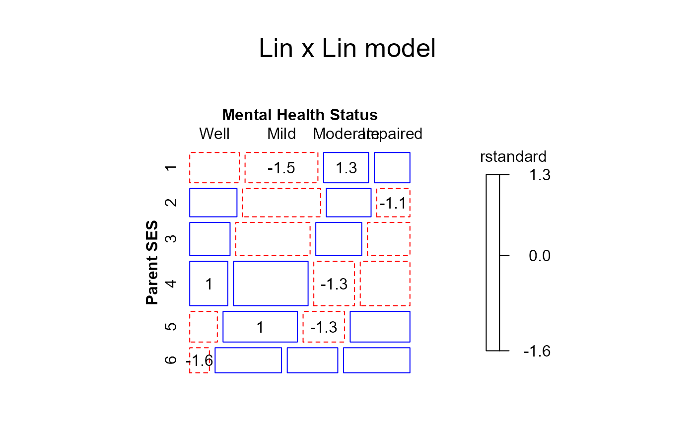
 # fit linear x linear (uniform) association. Use integer scores for rows/cols
Cscore <- as.numeric(Mental$ses)
Rscore <- as.numeric(Mental$mental)
linlin <- glm(Freq ~ mental + ses + Rscore:Cscore,
family = poisson, data = Mental)
mosaic(linlin,
formula = ~ses + mental,
residuals_type="rstandard",
labeling_args = long.labels,
labeling=labeling_residuals,
suppress=1,
gp=shading_Friendly,
main="Lin x Lin model")
# fit linear x linear (uniform) association. Use integer scores for rows/cols
Cscore <- as.numeric(Mental$ses)
Rscore <- as.numeric(Mental$mental)
linlin <- glm(Freq ~ mental + ses + Rscore:Cscore,
family = poisson, data = Mental)
mosaic(linlin,
formula = ~ses + mental,
residuals_type="rstandard",
labeling_args = long.labels,
labeling=labeling_residuals,
suppress=1,
gp=shading_Friendly,
main="Lin x Lin model")
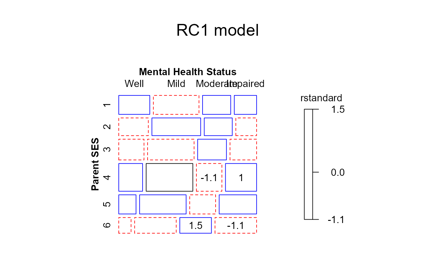
 ## Goodman Row-Column association model fits even better (deviance 3.57, df 8)
if (require(gnm)) {
Mental$mental <- C(Mental$mental, treatment)
Mental$ses <- C(Mental$ses, treatment)
RC1model <- gnm(Freq ~ ses + mental + Mult(ses, mental),
family = poisson, data = Mental)
mosaic(RC1model,
formula = ~ses + mental,
residuals_type="rstandard",
labeling_args = long.labels,
labeling=labeling_residuals,
suppress=1,
gp=shading_Friendly,
main="RC1 model")
}
#> Initialising
#> Running start-up iterations..
#> Running main iterations........
#> Done
## Goodman Row-Column association model fits even better (deviance 3.57, df 8)
if (require(gnm)) {
Mental$mental <- C(Mental$mental, treatment)
Mental$ses <- C(Mental$ses, treatment)
RC1model <- gnm(Freq ~ ses + mental + Mult(ses, mental),
family = poisson, data = Mental)
mosaic(RC1model,
formula = ~ses + mental,
residuals_type="rstandard",
labeling_args = long.labels,
labeling=labeling_residuals,
suppress=1,
gp=shading_Friendly,
main="RC1 model")
}
#> Initialising
#> Running start-up iterations..
#> Running main iterations........
#> Done
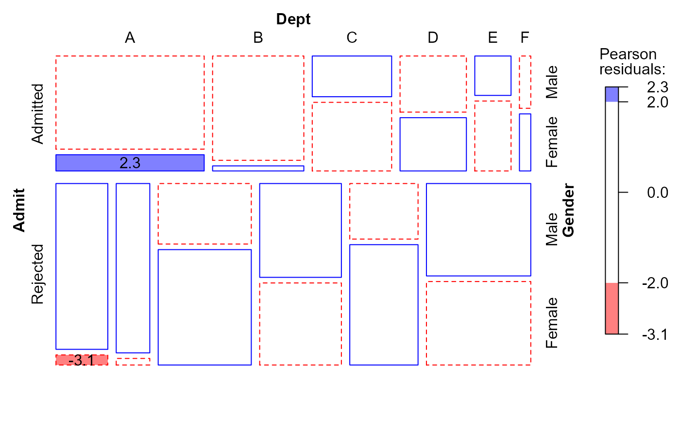
 ############# UCB Admissions data, fit using glm()
structable(Dept ~ Admit+Gender,UCBAdmissions)
#> Dept A B C D E F
#> Admit Gender
#> Admitted Male 512 353 120 138 53 22
#> Female 89 17 202 131 94 24
#> Rejected Male 313 207 205 279 138 351
#> Female 19 8 391 244 299 317
berkeley <- as.data.frame(UCBAdmissions)
berk.glm1 <- glm(Freq ~ Dept * (Gender+Admit), data=berkeley, family="poisson")
summary(berk.glm1)
#>
#> Call:
#> glm(formula = Freq ~ Dept * (Gender + Admit), family = "poisson",
#> data = berkeley)
#>
#> Coefficients:
#> Estimate Std. Error z value Pr(>|z|)
#> (Intercept) 6.27557 0.04248 147.744 < 2e-16 ***
#> DeptB -0.40575 0.06770 -5.993 2.06e-09 ***
#> DeptC -1.53939 0.08305 -18.536 < 2e-16 ***
#> DeptD -1.32234 0.08159 -16.207 < 2e-16 ***
#> DeptE -2.40277 0.11014 -21.816 < 2e-16 ***
#> DeptF -3.09624 0.15756 -19.652 < 2e-16 ***
#> GenderFemale -2.03325 0.10233 -19.870 < 2e-16 ***
#> AdmitRejected -0.59346 0.06838 -8.679 < 2e-16 ***
#> DeptB:GenderFemale -1.07581 0.22860 -4.706 2.52e-06 ***
#> DeptC:GenderFemale 2.63462 0.12343 21.345 < 2e-16 ***
#> DeptD:GenderFemale 1.92709 0.12464 15.461 < 2e-16 ***
#> DeptE:GenderFemale 2.75479 0.13510 20.391 < 2e-16 ***
#> DeptF:GenderFemale 1.94356 0.12683 15.325 < 2e-16 ***
#> DeptB:AdmitRejected 0.05059 0.10968 0.461 0.645
#> DeptC:AdmitRejected 1.20915 0.09726 12.432 < 2e-16 ***
#> DeptD:AdmitRejected 1.25833 0.10152 12.395 < 2e-16 ***
#> DeptE:AdmitRejected 1.68296 0.11733 14.343 < 2e-16 ***
#> DeptF:AdmitRejected 3.26911 0.16707 19.567 < 2e-16 ***
#> ---
#> Signif. codes: 0 ‘***’ 0.001 ‘**’ 0.01 ‘*’ 0.05 ‘.’ 0.1 ‘ ’ 1
#>
#> (Dispersion parameter for poisson family taken to be 1)
#>
#> Null deviance: 2650.095 on 23 degrees of freedom
#> Residual deviance: 21.736 on 6 degrees of freedom
#> AIC: 216.8
#>
#> Number of Fisher Scoring iterations: 4
#>
mosaic(berk.glm1,
gp=shading_Friendly,
labeling=labeling_residuals,
formula=~Admit+Dept+Gender)
############# UCB Admissions data, fit using glm()
structable(Dept ~ Admit+Gender,UCBAdmissions)
#> Dept A B C D E F
#> Admit Gender
#> Admitted Male 512 353 120 138 53 22
#> Female 89 17 202 131 94 24
#> Rejected Male 313 207 205 279 138 351
#> Female 19 8 391 244 299 317
berkeley <- as.data.frame(UCBAdmissions)
berk.glm1 <- glm(Freq ~ Dept * (Gender+Admit), data=berkeley, family="poisson")
summary(berk.glm1)
#>
#> Call:
#> glm(formula = Freq ~ Dept * (Gender + Admit), family = "poisson",
#> data = berkeley)
#>
#> Coefficients:
#> Estimate Std. Error z value Pr(>|z|)
#> (Intercept) 6.27557 0.04248 147.744 < 2e-16 ***
#> DeptB -0.40575 0.06770 -5.993 2.06e-09 ***
#> DeptC -1.53939 0.08305 -18.536 < 2e-16 ***
#> DeptD -1.32234 0.08159 -16.207 < 2e-16 ***
#> DeptE -2.40277 0.11014 -21.816 < 2e-16 ***
#> DeptF -3.09624 0.15756 -19.652 < 2e-16 ***
#> GenderFemale -2.03325 0.10233 -19.870 < 2e-16 ***
#> AdmitRejected -0.59346 0.06838 -8.679 < 2e-16 ***
#> DeptB:GenderFemale -1.07581 0.22860 -4.706 2.52e-06 ***
#> DeptC:GenderFemale 2.63462 0.12343 21.345 < 2e-16 ***
#> DeptD:GenderFemale 1.92709 0.12464 15.461 < 2e-16 ***
#> DeptE:GenderFemale 2.75479 0.13510 20.391 < 2e-16 ***
#> DeptF:GenderFemale 1.94356 0.12683 15.325 < 2e-16 ***
#> DeptB:AdmitRejected 0.05059 0.10968 0.461 0.645
#> DeptC:AdmitRejected 1.20915 0.09726 12.432 < 2e-16 ***
#> DeptD:AdmitRejected 1.25833 0.10152 12.395 < 2e-16 ***
#> DeptE:AdmitRejected 1.68296 0.11733 14.343 < 2e-16 ***
#> DeptF:AdmitRejected 3.26911 0.16707 19.567 < 2e-16 ***
#> ---
#> Signif. codes: 0 ‘***’ 0.001 ‘**’ 0.01 ‘*’ 0.05 ‘.’ 0.1 ‘ ’ 1
#>
#> (Dispersion parameter for poisson family taken to be 1)
#>
#> Null deviance: 2650.095 on 23 degrees of freedom
#> Residual deviance: 21.736 on 6 degrees of freedom
#> AIC: 216.8
#>
#> Number of Fisher Scoring iterations: 4
#>
mosaic(berk.glm1,
gp=shading_Friendly,
labeling=labeling_residuals,
formula=~Admit+Dept+Gender)
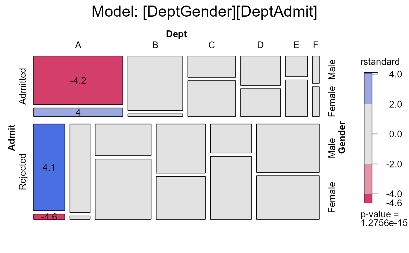
 # the same, displaying studentized residuals;
# note use of formula to reorder factors in the mosaic
mosaic(berk.glm1,
residuals_type="rstandard",
labeling=labeling_residuals,
shade=TRUE,
formula=~Admit+Dept+Gender,
main="Model: [DeptGender][DeptAdmit]")
# the same, displaying studentized residuals;
# note use of formula to reorder factors in the mosaic
mosaic(berk.glm1,
residuals_type="rstandard",
labeling=labeling_residuals,
shade=TRUE,
formula=~Admit+Dept+Gender,
main="Model: [DeptGender][DeptAdmit]")
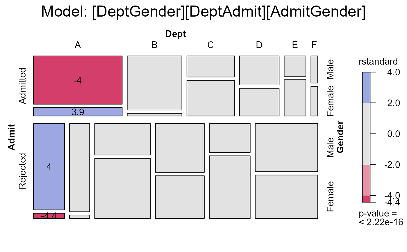
 ## all two-way model
berk.glm2 <- glm(Freq ~ (Dept + Gender + Admit)^2, data=berkeley, family="poisson")
summary(berk.glm2)
#>
#> Call:
#> glm(formula = Freq ~ (Dept + Gender + Admit)^2, family = "poisson",
#> data = berkeley)
#>
#> Coefficients:
#> Estimate Std. Error z value Pr(>|z|)
#> (Intercept) 6.27150 0.04271 146.855 < 2e-16 ***
#> DeptB -0.40322 0.06784 -5.944 2.78e-09 ***
#> DeptC -1.57790 0.08949 -17.632 < 2e-16 ***
#> DeptD -1.35000 0.08526 -15.834 < 2e-16 ***
#> DeptE -2.44982 0.11755 -20.840 < 2e-16 ***
#> DeptF -3.13787 0.16174 -19.401 < 2e-16 ***
#> GenderFemale -1.99859 0.10593 -18.866 < 2e-16 ***
#> AdmitRejected -0.58205 0.06899 -8.436 < 2e-16 ***
#> DeptB:GenderFemale -1.07482 0.22861 -4.701 2.58e-06 ***
#> DeptC:GenderFemale 2.66513 0.12609 21.137 < 2e-16 ***
#> DeptD:GenderFemale 1.95832 0.12734 15.379 < 2e-16 ***
#> DeptE:GenderFemale 2.79519 0.13925 20.073 < 2e-16 ***
#> DeptF:GenderFemale 2.00232 0.13571 14.754 < 2e-16 ***
#> DeptB:AdmitRejected 0.04340 0.10984 0.395 0.693
#> DeptC:AdmitRejected 1.26260 0.10663 11.841 < 2e-16 ***
#> DeptD:AdmitRejected 1.29461 0.10582 12.234 < 2e-16 ***
#> DeptE:AdmitRejected 1.73931 0.12611 13.792 < 2e-16 ***
#> DeptF:AdmitRejected 3.30648 0.16998 19.452 < 2e-16 ***
#> GenderFemale:AdmitRejected -0.09987 0.08085 -1.235 0.217
#> ---
#> Signif. codes: 0 ‘***’ 0.001 ‘**’ 0.01 ‘*’ 0.05 ‘.’ 0.1 ‘ ’ 1
#>
#> (Dispersion parameter for poisson family taken to be 1)
#>
#> Null deviance: 2650.095 on 23 degrees of freedom
#> Residual deviance: 20.204 on 5 degrees of freedom
#> AIC: 217.26
#>
#> Number of Fisher Scoring iterations: 4
#>
mosaic(berk.glm2,
residuals_type="rstandard",
labeling = labeling_residuals,
shade=TRUE,
formula=~Admit+Dept+Gender,
main="Model: [DeptGender][DeptAdmit][AdmitGender]")
## all two-way model
berk.glm2 <- glm(Freq ~ (Dept + Gender + Admit)^2, data=berkeley, family="poisson")
summary(berk.glm2)
#>
#> Call:
#> glm(formula = Freq ~ (Dept + Gender + Admit)^2, family = "poisson",
#> data = berkeley)
#>
#> Coefficients:
#> Estimate Std. Error z value Pr(>|z|)
#> (Intercept) 6.27150 0.04271 146.855 < 2e-16 ***
#> DeptB -0.40322 0.06784 -5.944 2.78e-09 ***
#> DeptC -1.57790 0.08949 -17.632 < 2e-16 ***
#> DeptD -1.35000 0.08526 -15.834 < 2e-16 ***
#> DeptE -2.44982 0.11755 -20.840 < 2e-16 ***
#> DeptF -3.13787 0.16174 -19.401 < 2e-16 ***
#> GenderFemale -1.99859 0.10593 -18.866 < 2e-16 ***
#> AdmitRejected -0.58205 0.06899 -8.436 < 2e-16 ***
#> DeptB:GenderFemale -1.07482 0.22861 -4.701 2.58e-06 ***
#> DeptC:GenderFemale 2.66513 0.12609 21.137 < 2e-16 ***
#> DeptD:GenderFemale 1.95832 0.12734 15.379 < 2e-16 ***
#> DeptE:GenderFemale 2.79519 0.13925 20.073 < 2e-16 ***
#> DeptF:GenderFemale 2.00232 0.13571 14.754 < 2e-16 ***
#> DeptB:AdmitRejected 0.04340 0.10984 0.395 0.693
#> DeptC:AdmitRejected 1.26260 0.10663 11.841 < 2e-16 ***
#> DeptD:AdmitRejected 1.29461 0.10582 12.234 < 2e-16 ***
#> DeptE:AdmitRejected 1.73931 0.12611 13.792 < 2e-16 ***
#> DeptF:AdmitRejected 3.30648 0.16998 19.452 < 2e-16 ***
#> GenderFemale:AdmitRejected -0.09987 0.08085 -1.235 0.217
#> ---
#> Signif. codes: 0 ‘***’ 0.001 ‘**’ 0.01 ‘*’ 0.05 ‘.’ 0.1 ‘ ’ 1
#>
#> (Dispersion parameter for poisson family taken to be 1)
#>
#> Null deviance: 2650.095 on 23 degrees of freedom
#> Residual deviance: 20.204 on 5 degrees of freedom
#> AIC: 217.26
#>
#> Number of Fisher Scoring iterations: 4
#>
mosaic(berk.glm2,
residuals_type="rstandard",
labeling = labeling_residuals,
shade=TRUE,
formula=~Admit+Dept+Gender,
main="Model: [DeptGender][DeptAdmit][AdmitGender]")
 anova(berk.glm1, berk.glm2, test="Chisq")
#> Analysis of Deviance Table
#>
#> Model 1: Freq ~ Dept * (Gender + Admit)
#> Model 2: Freq ~ (Dept + Gender + Admit)^2
#> Resid. Df Resid. Dev Df Deviance Pr(>Chi)
#> 1 6 21.735
#> 2 5 20.204 1 1.5312 0.2159
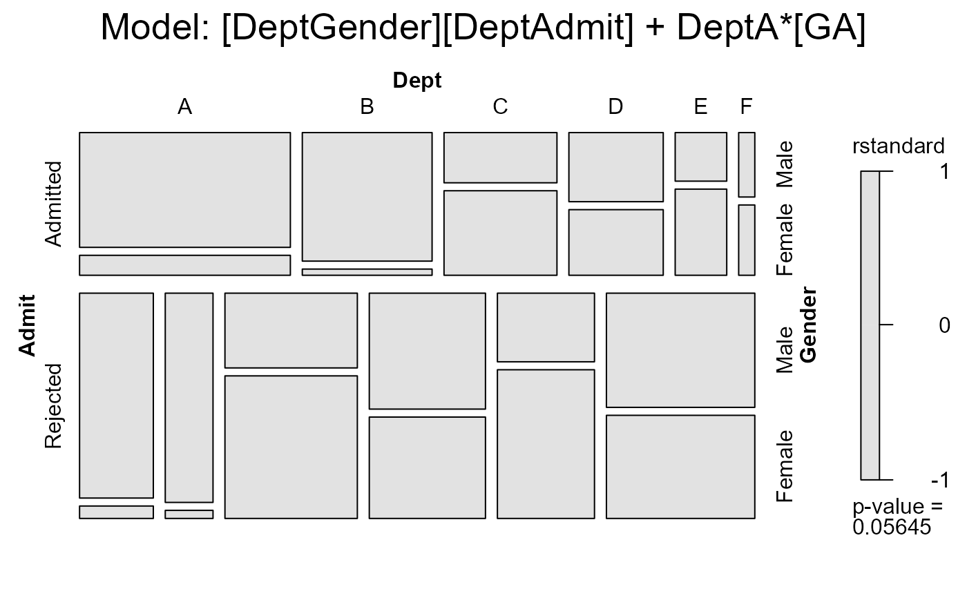
# Add 1 df term for association of [GenderAdmit] only in Dept A
berkeley <- within(berkeley,
dept1AG <- (Dept=='A')*(Gender=='Female')*(Admit=='Admitted'))
berkeley[1:6,]
#> Admit Gender Dept Freq dept1AG
#> 1 Admitted Male A 512 0
#> 2 Rejected Male A 313 0
#> 3 Admitted Female A 89 1
#> 4 Rejected Female A 19 0
#> 5 Admitted Male B 353 0
#> 6 Rejected Male B 207 0
berk.glm3 <- glm(Freq ~ Dept * (Gender+Admit) + dept1AG, data=berkeley, family="poisson")
summary(berk.glm3)
#>
#> Call:
#> glm(formula = Freq ~ Dept * (Gender + Admit) + dept1AG, family = "poisson",
#> data = berkeley)
#>
#> Coefficients:
#> Estimate Std. Error z value Pr(>|z|)
#> (Intercept) 6.23832 0.04419 141.157 < 2e-16 ***
#> DeptB -0.36850 0.06879 -5.357 8.47e-08 ***
#> DeptC -1.50215 0.08394 -17.895 < 2e-16 ***
#> DeptD -1.28509 0.08250 -15.577 < 2e-16 ***
#> DeptE -2.36552 0.11081 -21.347 < 2e-16 ***
#> DeptF -3.05899 0.15803 -19.357 < 2e-16 ***
#> GenderFemale -2.80176 0.23628 -11.858 < 2e-16 ***
#> AdmitRejected -0.49212 0.07175 -6.859 6.94e-12 ***
#> dept1AG 1.05208 0.26271 4.005 6.21e-05 ***
#> DeptB:GenderFemale -0.30730 0.31243 -0.984 0.325
#> DeptC:GenderFemale 3.40313 0.24615 13.825 < 2e-16 ***
#> DeptD:GenderFemale 2.69560 0.24676 10.924 < 2e-16 ***
#> DeptE:GenderFemale 3.52330 0.25220 13.970 < 2e-16 ***
#> DeptF:GenderFemale 2.71207 0.24787 10.941 < 2e-16 ***
#> DeptB:AdmitRejected -0.05074 0.11181 -0.454 0.650
#> DeptC:AdmitRejected 1.10781 0.09966 11.116 < 2e-16 ***
#> DeptD:AdmitRejected 1.15699 0.10381 11.145 < 2e-16 ***
#> DeptE:AdmitRejected 1.58162 0.11933 13.254 < 2e-16 ***
#> DeptF:AdmitRejected 3.16777 0.16848 18.803 < 2e-16 ***
#> ---
#> Signif. codes: 0 ‘***’ 0.001 ‘**’ 0.01 ‘*’ 0.05 ‘.’ 0.1 ‘ ’ 1
#>
#> (Dispersion parameter for poisson family taken to be 1)
#>
#> Null deviance: 2650.0952 on 23 degrees of freedom
#> Residual deviance: 2.6815 on 5 degrees of freedom
#> AIC: 199.74
#>
#> Number of Fisher Scoring iterations: 3
#>
mosaic(berk.glm3,
residuals_type = "rstandard",
labeling = labeling_residuals,
shade=TRUE,
formula = ~Admit+Dept+Gender,
main = "Model: [DeptGender][DeptAdmit] + DeptA*[GA]")
anova(berk.glm1, berk.glm2, test="Chisq")
#> Analysis of Deviance Table
#>
#> Model 1: Freq ~ Dept * (Gender + Admit)
#> Model 2: Freq ~ (Dept + Gender + Admit)^2
#> Resid. Df Resid. Dev Df Deviance Pr(>Chi)
#> 1 6 21.735
#> 2 5 20.204 1 1.5312 0.2159
# Add 1 df term for association of [GenderAdmit] only in Dept A
berkeley <- within(berkeley,
dept1AG <- (Dept=='A')*(Gender=='Female')*(Admit=='Admitted'))
berkeley[1:6,]
#> Admit Gender Dept Freq dept1AG
#> 1 Admitted Male A 512 0
#> 2 Rejected Male A 313 0
#> 3 Admitted Female A 89 1
#> 4 Rejected Female A 19 0
#> 5 Admitted Male B 353 0
#> 6 Rejected Male B 207 0
berk.glm3 <- glm(Freq ~ Dept * (Gender+Admit) + dept1AG, data=berkeley, family="poisson")
summary(berk.glm3)
#>
#> Call:
#> glm(formula = Freq ~ Dept * (Gender + Admit) + dept1AG, family = "poisson",
#> data = berkeley)
#>
#> Coefficients:
#> Estimate Std. Error z value Pr(>|z|)
#> (Intercept) 6.23832 0.04419 141.157 < 2e-16 ***
#> DeptB -0.36850 0.06879 -5.357 8.47e-08 ***
#> DeptC -1.50215 0.08394 -17.895 < 2e-16 ***
#> DeptD -1.28509 0.08250 -15.577 < 2e-16 ***
#> DeptE -2.36552 0.11081 -21.347 < 2e-16 ***
#> DeptF -3.05899 0.15803 -19.357 < 2e-16 ***
#> GenderFemale -2.80176 0.23628 -11.858 < 2e-16 ***
#> AdmitRejected -0.49212 0.07175 -6.859 6.94e-12 ***
#> dept1AG 1.05208 0.26271 4.005 6.21e-05 ***
#> DeptB:GenderFemale -0.30730 0.31243 -0.984 0.325
#> DeptC:GenderFemale 3.40313 0.24615 13.825 < 2e-16 ***
#> DeptD:GenderFemale 2.69560 0.24676 10.924 < 2e-16 ***
#> DeptE:GenderFemale 3.52330 0.25220 13.970 < 2e-16 ***
#> DeptF:GenderFemale 2.71207 0.24787 10.941 < 2e-16 ***
#> DeptB:AdmitRejected -0.05074 0.11181 -0.454 0.650
#> DeptC:AdmitRejected 1.10781 0.09966 11.116 < 2e-16 ***
#> DeptD:AdmitRejected 1.15699 0.10381 11.145 < 2e-16 ***
#> DeptE:AdmitRejected 1.58162 0.11933 13.254 < 2e-16 ***
#> DeptF:AdmitRejected 3.16777 0.16848 18.803 < 2e-16 ***
#> ---
#> Signif. codes: 0 ‘***’ 0.001 ‘**’ 0.01 ‘*’ 0.05 ‘.’ 0.1 ‘ ’ 1
#>
#> (Dispersion parameter for poisson family taken to be 1)
#>
#> Null deviance: 2650.0952 on 23 degrees of freedom
#> Residual deviance: 2.6815 on 5 degrees of freedom
#> AIC: 199.74
#>
#> Number of Fisher Scoring iterations: 3
#>
mosaic(berk.glm3,
residuals_type = "rstandard",
labeling = labeling_residuals,
shade=TRUE,
formula = ~Admit+Dept+Gender,
main = "Model: [DeptGender][DeptAdmit] + DeptA*[GA]")
 # compare models
anova(berk.glm1, berk.glm3, test="Chisq")
#> Analysis of Deviance Table
#>
#> Model 1: Freq ~ Dept * (Gender + Admit)
#> Model 2: Freq ~ Dept * (Gender + Admit) + dept1AG
#> Resid. Df Resid. Dev Df Deviance Pr(>Chi)
#> 1 6 21.7355
#> 2 5 2.6815 1 19.054 1.271e-05 ***
#> ---
#> Signif. codes: 0 ‘***’ 0.001 ‘**’ 0.01 ‘*’ 0.05 ‘.’ 0.1 ‘ ’ 1
# compare models
anova(berk.glm1, berk.glm3, test="Chisq")
#> Analysis of Deviance Table
#>
#> Model 1: Freq ~ Dept * (Gender + Admit)
#> Model 2: Freq ~ Dept * (Gender + Admit) + dept1AG
#> Resid. Df Resid. Dev Df Deviance Pr(>Chi)
#> 1 6 21.7355
#> 2 5 2.6815 1 19.054 1.271e-05 ***
#> ---
#> Signif. codes: 0 ‘***’ 0.001 ‘**’ 0.01 ‘*’ 0.05 ‘.’ 0.1 ‘ ’ 1