Version 0.4.1; documentation built for pkgdown 2026-03-08
The nestedLogit package provides functions for fitting nested dichotomy logistic regression models for a polytomous response (with categories), such as:
- support for political party in Canada (PC, Liberal, NDP, Green, BQ),
- preferred mode of transport (foot, bus, bike, train, plane),
- womens’ working status (not working, part-time, full-time).
The figure below shows two different ways that a -category polytomous response can be decomposed as three () nested dichotomies among the levels.
- In the case shown at the left of the figure, the response categories are divided first as vs. . Then these compound categories are subdivided as the dichotomies vs. and as vs. .
- Alternatively, as shown at the right of the figure, the response categories are divided progressively: first as vs. ; next as vs. ; and and finally vs. .
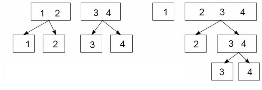
Nested dichotomies: The boxes show two different ways a four-category response can be represented as three nested dichotomies.
⚙️ Related models for a polytomous response
The basic model for this situation ( response categories) is the standard multinomial logistic model (fit by: e.g., nnet::multinom()) which compares response categories to a reference level.
When you can think of the differences among the response categories as a set nested comparisons among subsets of the categories, the approach of nested dichotomies is simpler, because:
- Nested dichotomies are statistically independent, and hence:
- the likelihood chi-square statistics for the sub-models are additive;
- they provide an additive decomposition of tests for the overall polytomous response.
- You can think of this as breaking up the overall question of “How do the response categories differ?” into non-overlapping sub-questions that answer the global one.
When the dichotomies make sense substantively, this method can be a simpler alternative to the standard multinomial logistic model which compares response categories to a reference level. This choice is similar to using orthogonal contrasts among factor categories in an ANOVA, as opposed to using the default reference-level coding.
The benefit is that, with nested logit models, you get to ask substantively more interesting questions directly than you can with the multinomial logit model. The results (for overall tests) are nearly equivalent. But, you get to think better about your problem with the nested logit model.
Ordered categories
Note that when the response categories are ordered, as in education attained: “HS” < “College” < “BA” < “MA” < “PhD”, another attractive model is the proportional odds model (e.g., fit by MASS::polr()). This is a simpler model, but achieves that simplicity by making the additional assumption that the coefficients for the predictors are the same for all categories.
🚀 Installation
You can install the current published version (0.4.0) from CRAN, or the development version (0.4.1) from either R-universe or Github
| CRAN version | install.packages("nestedLogit") |
| R-universe | install.packages('nestedLogit', repos = 'https://friendly.r-universe.dev') |
| Github | remotes::install_github("friendly/nestedLogit") |
✨ Package overview
The package provides one main function, nestedLogit() for fitting the set of binary logistic regression models for a polytomous response with levels. It has the full suited of methods associated with glm() and other model fitting methods.
What is novel in R software design are aspects of a grammar for specifying dichotomies in model formulas, and the idea of fitting an overall model, which is composed of submodels that we want to also consider, test, plot, …
Specifying dichotomies
The essential idea here is to have a simple notation expressing a dichotomy among response levels, like {{A, B}, {C, D}}, and then a way to specify a collection of of these that can be used productively in data analysis and visualization.
In the nestedLogit package these can be specified using helper functions:
-
dichotomy(): constructs a single dichotomy among the levels of a response factor; -
logits(): creates the set of dichotomies, typically usingdichotomy()for each. -
continuationLogits(): provides a convenient way to generate all dichotomies for an ordered response.
For instance, a 4-category response, with levels A, B, C, D, and successive binary splits for the dichotomies of interest could be specified as:
(ABCD <-
  logits(AB.CD = dichotomy(c("A", "B"), c("C", "D")),
           A.B = dichotomy("A", "B"),
           C.D = dichotomy("C", "D")
         )
)
#> AB.CD: {A, B} vs. {C, D}
#> A.B: {A} vs. {B}
#> C.D: {C} vs. {D}
These dichotomies are effectively a tree structure of lists, which can be displayed simply using lobstr::tree().
lobstr::tree(ABCD)
#> S3<dichotomies>
#> ├─AB.CD: <list>
#> │ ├─<chr [2]>"A", "B"
#> │ └─<chr [2]>"C", "D"
#> ├─A.B: <list>
#> │ ├─"A"
#> │ └─"B"
#> └─C.D: <list>
#>   ├─"C"
#>   └─"D"
Alternatively, the nested dichotomies can be specified more compactly as a nested (i.e., recursive) list with optionally named elements. For example, where people might choose a method of transportation among the categories plane, train, bus, car, a sensible set of three dichotomies could be specified as:
transport <- list(
  air = "plane",
  ground = list(
    public = list("train", "bus"),
    private = "car"
  ))

lobstr::tree(transport)
#> <list>
#> ├─air: "plane"
#> └─ground: <list>
#>   ├─public: <list>
#>   │ ├─"train"
#>   │ └─"bus"
#>   └─private: "car"
There are also methods including as.matrix.dichotomies(), as.character.dichotomies() to facilitate working with dichotomies objects in other representations. The ABCD example above corresponds to the matrix below, whose rows represent the dichotomies and columns are the response levels:
as.matrix(ABCD)
#>        A  B  C  D
#> AB.CD  0  0  1  1
#> A.B    0  1 NA NA
#> C.D   NA NA  0  1

as.character(ABCD)
#> [1] "AB.CD = {{A B}} {{C D}}; A.B = {{A}} {{B}}; C.D = {{C}} {{D}}"
The result of nestedLogit() is an object of class "nestedLogit". It contains the set of glm() models fit to the dichotomies.
Methods
As befits a model-fitting function, the package defines a nearly complete set of methods for "nestedLogit" objects:
-
print()andsummary()print the results for each of the submodels. -
update()re-fits the model, allowing changes to the modelformula,data,subset, andcontrastsarguments. -
coef()returns the coefficients for the predictors in each dichotomy. -
vcov()returns the variance-covariance matrix of the coefficients -
predict()computes predicted probabilities for the response categories, either for the cases in the data, which is equivalent tofitted(), or for arbitrary combinations of the predictors; the latter is useful for producing plots to aid interpretation. -
confint()calculates confidence intervals for the predicted probabilities or predicted logits. -
as.data.frame()method for predicted probabilities and logits converts these to long format for use withggplot2. -
glance()andtidy()are extensions ofbroom::glance.glm()andbroom::tidy.glm()to obtain compact summaries of a"nestedLogit"model object. -
plot()provides basic plots of the predicted probabilities over a range of values of the predictor variables. -
models()is an extractor function for the binary logit models in the"nestedLogit"object -
Effect()calculates marginal effects collapsed over some variable(s) for the purpose of making effect plots.
These functions are supplemented by various methods for testing hypotheses about and comparing nested-logit models:
-
anova()provides analysis-of-deviance Type I (sequential) tests for each dichotomy and for the combined model. When given a sequence of model objects,anova()tests the models against one another in the order specified. -
Anova()usescar::Anova()to provide analysis-of-deviance Type II or III (partial) tests for each dichotomy and for the combined model. -
linearHypothesis()usescar::linearHypothesis()to compute Wald tests for hypotheses about coefficients or their linear combinations. -
logLik()returns the log-likelihood and degrees of freedom for the nested-dichotomies logit model. - Through
logLik(), theAIC()andBIC()functions compute the Akaike and Bayesian information criteria model-comparison statistics. -
RSQ()computes a variety of pseudo (McFadden, CoxSnell, Nagelkerke, …) measures for nested logit models.
🎨 Examples
This example uses data on women’s labor force participation to fit a nested logit model for the response, partic, representing categories not.work, parttime and fulltime for 263 women from a 1977 survey in Canada. This dataset is explored in more detail in the package vignette, vignette("nestedLogits", package = "nestedLogit").
A model for the complete polytomy can be specified as two nested dichotomies, using helper functions dichotomy() and logits(), as shown in the example that follows:
-
work: {not.work} vs. {parttime, fulltime} -
full: {parttime} vs. {fulltime}, but only for those working
nestedLogit() effectively fits each of these dichotomies as logistic regression models via glm(..., family = binomial)
data(Womenlf, package = "carData")

# Use `logits()` and `dichotomy()` to specify the comparisons of interest
comparisons <- logits(work=dichotomy("not.work",
                                     working=c("parttime", "fulltime")),
                      full=dichotomy("parttime", "fulltime"))

m <- nestedLogit(partic ~ hincome + children,
                 dichotomies = comparisons,
                 data=Womenlf)
coef(m)
#>                        work       full
#> (Intercept)      1.33582979  3.4777735
#> hincome         -0.04230843 -0.1072679
#> childrenpresent -1.57564843 -2.6514557
The "nestedLogit" object contains the components of the fitted model. The structure can be shown nicely using lobstr::tree():
m |> lobstr::tree(max_depth=1)
#> S3<nestedLogit>
#> ├─models: <list>...
#> ├─formula: S3<formula> partic ~ hincome + children...
#> ├─dichotomies: S3<dichotomies>...
#> ├─data: S3<data.frame>...
#> ├─data.name: <symbol> Womenlf
#> ├─subset: <NULL>
#> ├─contrasts: <NULL>
#> └─contrasts.print: "NULL"
The separate models for the work and full dichotomies can be extracted via models(). These are the binomial glm() models.
models(m) |> lobstr::tree(max_depth = 1)
#> <list>
#> ├─work: S3<glm/lm>...
#> └─full: S3<glm/lm>...
Anova() produces analysis of variance deviance tests for the terms in this model for each of the submodels, as well as for the combined responses of the polytomy. The LR Chisq and df for terms in the combined model are the sums of those for the submodels.
car::Anova(m)
#>
#>  Analysis of Deviance Tables (Type II tests)
#>
#> Response work: {not.work} vs. working{parttime, fulltime}
#>          LR Chisq Df Pr(>Chisq)
#> hincome    4.8264  1    0.02803 *
#> children  31.3229  1  2.185e-08 ***
#> ---
#> Signif. codes:  0 '***' 0.001 '**' 0.01 '*' 0.05 '.' 0.1 ' ' 1
#>
#>
#> Response full: {parttime} vs. {fulltime}
#>          LR Chisq Df Pr(>Chisq)
#> hincome     8.981  1   0.002728 **
#> children   32.136  1  1.437e-08 ***
#> ---
#> Signif. codes:  0 '***' 0.001 '**' 0.01 '*' 0.05 '.' 0.1 ' ' 1
#>
#>
#> Combined Responses
#>          LR Chisq Df Pr(>Chisq)
#> hincome    13.808  2   0.001004 **
#> children   63.459  2   1.66e-14 ***
#> ---
#> Signif. codes:  0 '***' 0.001 '**' 0.01 '*' 0.05 '.' 0.1 ' ' 1
Plots
A basic plot of predicted probabilities can be produced using the plot() method for "nestedLogit" objects. It can be called several times to give multi-panel plots. By default, a 95% pointwise confidence envelope is added to the plot. Here, they are plotted with conf.level = 0.68 to give std. error bounds.
op <- par(mfcol=c(1, 2), mar=c(4, 4, 3, 1) + 0.1)
plot(m, "hincome", list(children="absent"),
     conf.level = 0.68,
     xlab="Husband's Income", legend=FALSE)
plot(m, "hincome", list(children="present"),
     conf.level = 0.68,
     xlab="Husband's Income")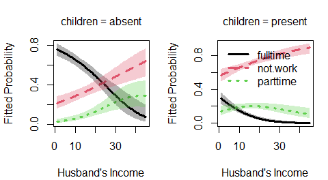
📜 Vignettes
A more general discussion of nested dichotomies logistic regression and detailed examples can be found in
vignette("nestedLogit", package="nestedLogit")and in the pkgdown documentation.A variety of other plots can be produced using
ggplot(), as described in the vignette,vignette("plotting-ggplot")and in the pkgdown documentation.Figuring out how to calculate uncertainty estimates for nested logit models was solved John Fox. The vignette,
vignette("standard-errors"), describes the mathematics behind the calculation of standard errors using the delta method.A collection of other examples of datasets for which nested logit models are useful, described in
vignette("other-examples")and pkgdown documentation.
References
S. Fienberg (1980) The Analysis of Cross-Classified Categorical Data, 2nd Edition, MIT Press, Section 6.6.
J. Fox (2016) Applied Regression Analysis and Generalized Linear Models, 3rd Edition, Sage, Section 14.2.2.
M. Friendly and D. Meyers (2016) Discrete Data Analysis with R, CRC Press, Section 8.2.