Bartlett Data on Plum Root Cuttings

In an experiment to investigate the effect of cutting length (two levels) and planting time (two levels) on the survival of plum root cuttings, 240 cuttings were planted for each of the 2 x 2 combinations of these factors, and their survival was later recorded.

Bartlett (1935) used these data to illustrate a method for testing for no three-way interaction in a contingency table.

Usage

data(Bartlett)

Format

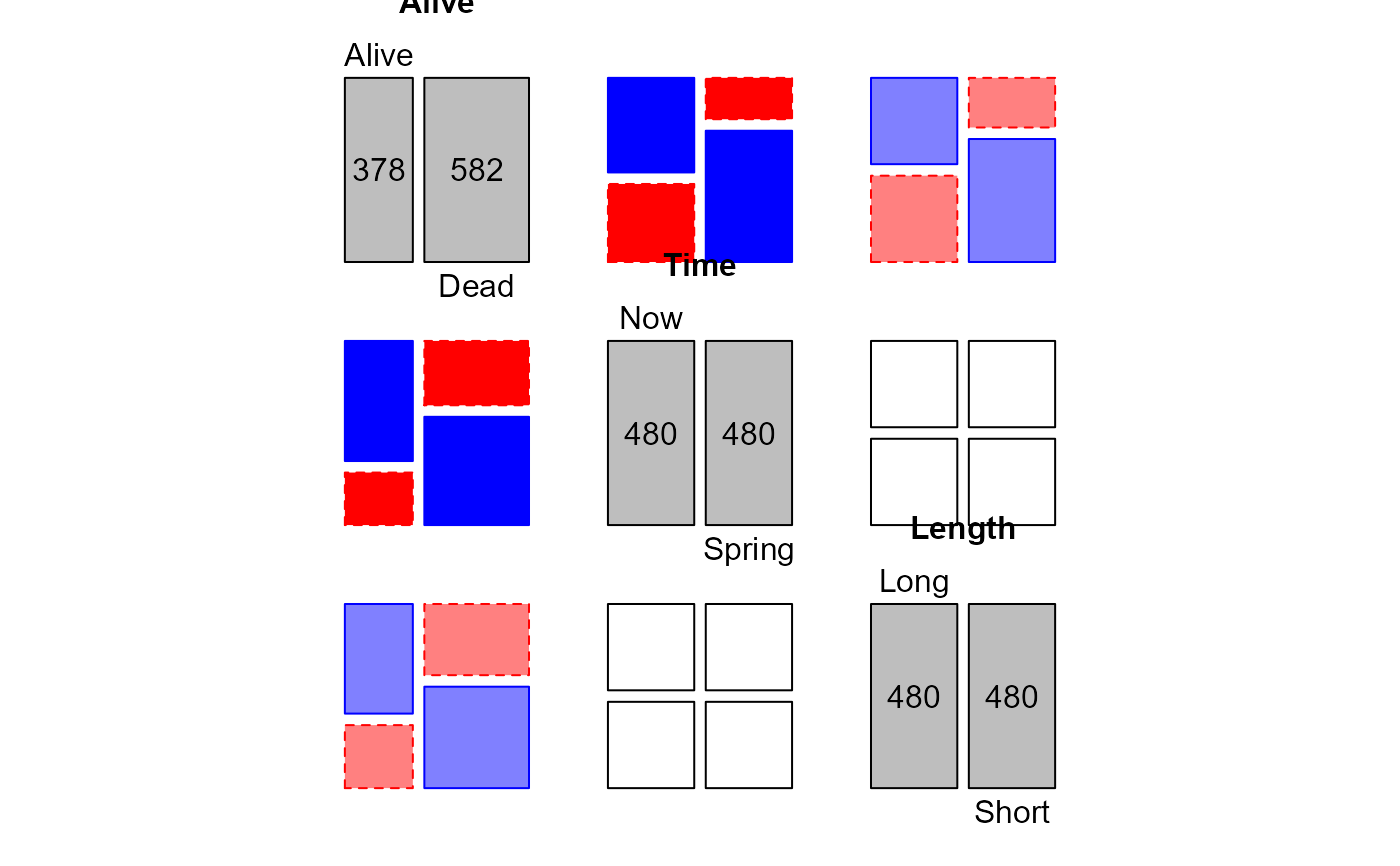
A 3-dimensional array resulting from cross-tabulating 3 variables for 960 observations. The variable names and their levels are:

No	Name	Levels
1	Alive	"Alive", "Dead"
2	Time	"Now", "Spring"
3	Length	"Long", "Short"

Source

Hand, D. and Daly, F. and Lunn, A. D.and McConway, K. J. and Ostrowski, E. (1994). A Handbook of Small Data Sets. London: Chapman & Hall, p. 15, # 19.

References

Bartlett, M. S. (1935). Contingency Table Interactions Journal of the Royal Statistical Society, Supplement, 1935, 2, 248-252.

Examples

data(Bartlett)

# measures of association
assocstats(Bartlett)
#> $`Length:Long`
#>                     X^2 df   P(> X^2)
#> Likelihood Ratio 43.873  1 3.5048e-11
#> Pearson          43.200  1 4.9421e-11
#> 
#> Phi-Coefficient   : 0.3 
#> Contingency Coeff.: 0.287 
#> Cramer's V        : 0.3 
#> 
#> $`Length:Short`
#>                     X^2 df   P(> X^2)
#> Likelihood Ratio 61.310  1 4.8850e-15
#> Pearson          58.744  1 1.7986e-14
#> 
#> Phi-Coefficient   : 0.35 
#> Contingency Coeff.: 0.33 
#> Cramer's V        : 0.35 
#> 
oddsratio(Bartlett)
#> log odds ratios for Alive and Time by Length 
#> 
#>     Long    Short 
#> 1.238078 1.690827 

# Test models

## Independence
MASS::loglm(formula = ~Alive + Time + Length, data = Bartlett)
#> Call:
#> MASS::loglm(formula = ~Alive + Time + Length, data = Bartlett)
#> 
#> Statistics:
#>                       X^2 df P(> X^2)
#> Likelihood Ratio 151.0193  4        0
#> Pearson          141.0527  4        0

## No three-way association
MASS::loglm(formula = ~(Alive + Time + Length)^2, data = Bartlett)
#> Call:
#> MASS::loglm(formula = ~(Alive + Time + Length)^2, data = Bartlett)
#> 
#> Statistics:
#>                       X^2 df  P(> X^2)
#> Likelihood Ratio 2.293841  1 0.1298882
#> Pearson          2.270373  1 0.1318681

# Use woolf_test() for a formal test of homogeneity of odds ratios
vcd::woolf_test(Bartlett)
#> 
#> 	Woolf-test on Homogeneity of Odds Ratios (no 3-Way assoc.)
#> 
#> data:  Bartlett
#> X-squared = 2.264, df = 1, p-value = 0.1324
#> 


# Plots
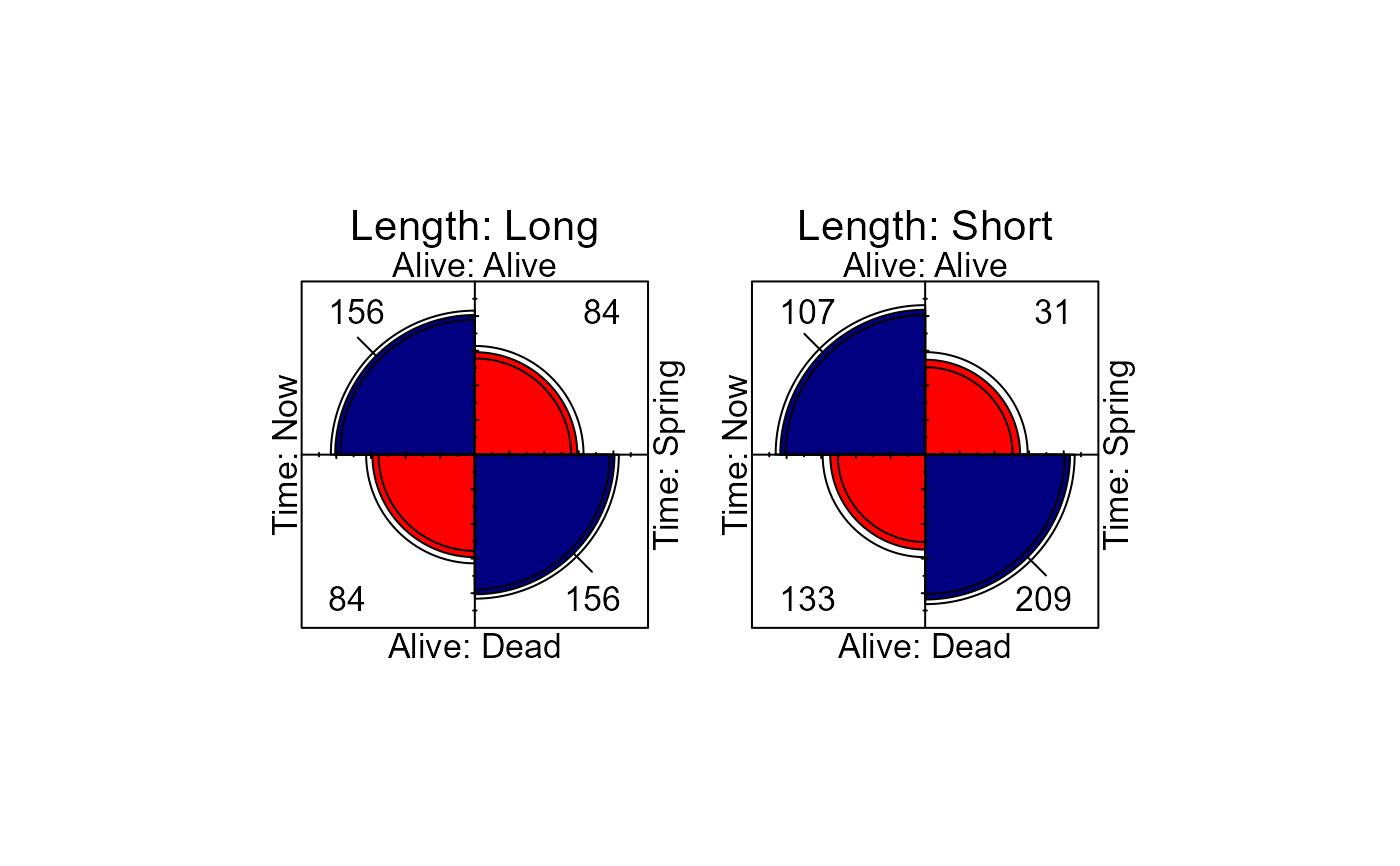
fourfold(Bartlett, mfrow=c(1,2))


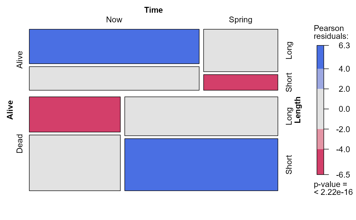
mosaic(Bartlett, shade=TRUE)

pairs(Bartlett, gp=shading_Friendly)