USA 1970 Draft Lottery Data

This data set gives the results of the 1970 US draft lottery, in the form of a data frame.

Usage

data(Draft1970)

Format

A data frame with 366 observations on the following 3 variables.

Day: day of the year, 1:366
Rank: draft priority rank of people born on that day
Month: an ordered factor with levels Jan < Feb ... < Dec

Details

The draft lottery was used to determine the order in which eligible men would be called to the Selective Service draft. The days of the year (including February 29) were represented by the numbers 1 through 366 written on slips of paper. The slips were placed in separate plastic capsules that were mixed in a shoebox and then dumped into a deep glass jar. Capsules were drawn from the jar one at a time.

The first number drawn was 258 (September 14), so all registrants with that birthday were assigned lottery number Rank 1. The second number drawn corresponded to April 24, and so forth. All men of draft age (born 1944 to 1950) who shared a birthdate would be called to serve at once. The first 195 birthdates drawn were later called to serve in the order they were drawn; the last of these was September 24.

Source

Starr, N. (1997). Nonrandom Risk: The 1970 Draft Lottery, Journal of Statistics Education, v.5, n.2 http://jse.amstat.org/v5n2/datasets.starr.html

References

Fienberg, S. E. (1971), "Randomization and Social Affairs: The 1970 Draft Lottery," Science, 171, 255-261.

https://en.wikipedia.org/wiki/Draft_lottery_(1969)

Examples

data(Draft1970)

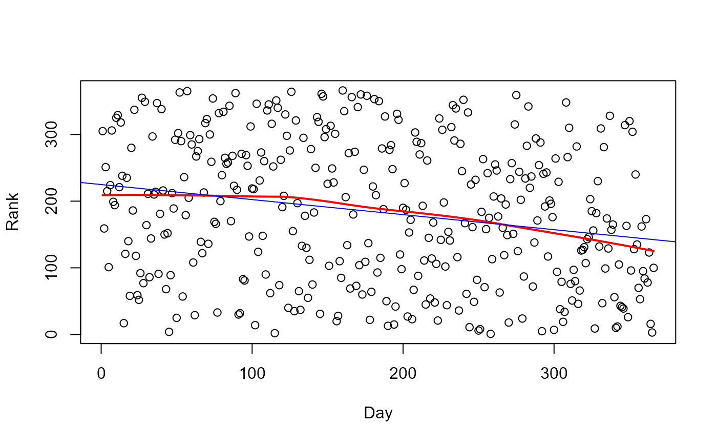
# scatterplot
plot(Rank ~ Day, data=Draft1970)
with(Draft1970, lines(lowess(Day, Rank), col="red", lwd=2))
abline(lm(Rank ~ Day, data=Draft1970), col="blue")

 
# boxplots
plot(Rank ~ Month, data=Draft1970, col="bisque")


lm(Rank ~ Month, data=Draft1970)
#> 
#> Call:
#> lm(formula = Rank ~ Month, data = Draft1970)
#> 
#> Coefficients:
#> (Intercept)      Month.L      Month.Q      Month.C      Month^4      Month^5  
#>     183.528      -84.330      -31.503        5.020      -20.904      -14.052  
#>     Month^6      Month^7      Month^8      Month^9     Month^10     Month^11  
#>       2.122        3.488       21.150        1.747       15.582        1.126  
#> 
anova(lm(Rank ~ Month, data=Draft1970))
#> Analysis of Variance Table
#> 
#> Response: Rank
#>            Df  Sum Sq Mean Sq F value  Pr(>F)   
#> Month      11  290507   26410  2.4634 0.00558 **
#> Residuals 354 3795120   10721                   
#> ---
#> Signif. codes:  0 '***' 0.001 '**' 0.01 '*' 0.05 '.' 0.1 ' ' 1

# make the table version
Draft1970$Risk <- cut(Draft1970$Rank, breaks=3, labels=c("High", "Med", "Low"))
with(Draft1970, table(Month, Risk))
#>      Risk
#> Month High Med Low
#>   Jan    9  12  10
#>   Feb    7  12  10
#>   Mar    5  10  16
#>   Apr    8   8  14
#>   May    9   7  15
#>   Jun   11   7  12
#>   Jul   12   7  12
#>   Aug   13   7  11
#>   Sep   10  15   5
#>   Oct    9  15   7
#>   Nov   12  12   6
#>   Dec   17  10   4