Hosmer-Lemeshow Goodness of Fit Test

The HLtest function computes the classical Hosmer-Lemeshow (1980) goodness of fit test for a binomial glm object in logistic regression

Usage

HLtest(model, g = 10)

# S3 method for class 'HLtest'
print(x, ...)

# S3 method for class 'HLtest'
summary(object, ...)

# S3 method for class 'HLtest'
rootogram(x, ...)

# S3 method for class 'HLtest'
plot(x, ...)

Arguments

model: A glm model object in the binomial family
g: Number of groups used to partition the fitted values for the GOF test.
x, object: A HLtest object
...: Other arguments passed down to methods

Value

A class HLtest object with the following components:

table: A data.frame describing the results of partitioning the data into g groups with the following columns: cut, total, obs, exp, chi
chisq: The chisquare statistics
df: Degrees of freedom
p.value: p value
groups: Number of groups
call: model call

%% ...

Details

The general idea is to assesses whether or not the observed event rates match expected event rates in subgroups of the model population. The Hosmer-Lemeshow test specifically identifies subgroups as the deciles of fitted event values, or other quantiles as determined by the g argument. Given these subgroups, a simple chisquare test on g-2 df is used.

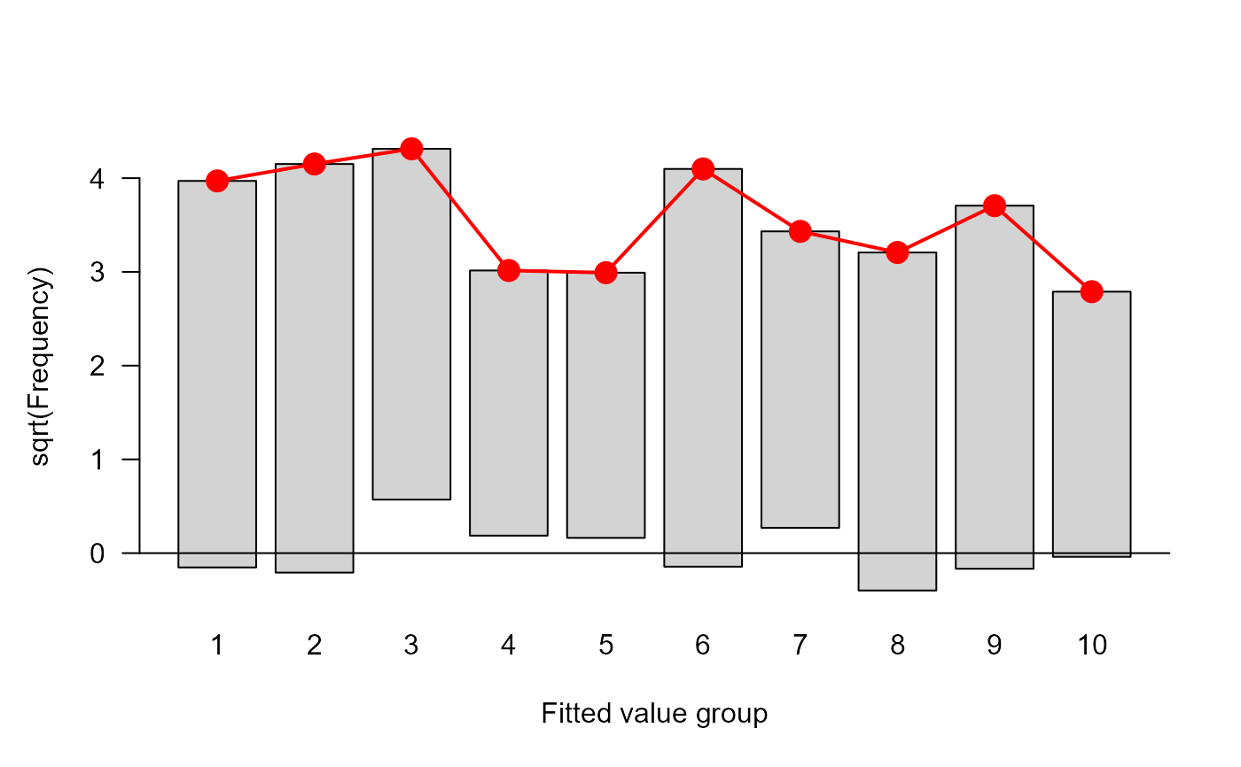
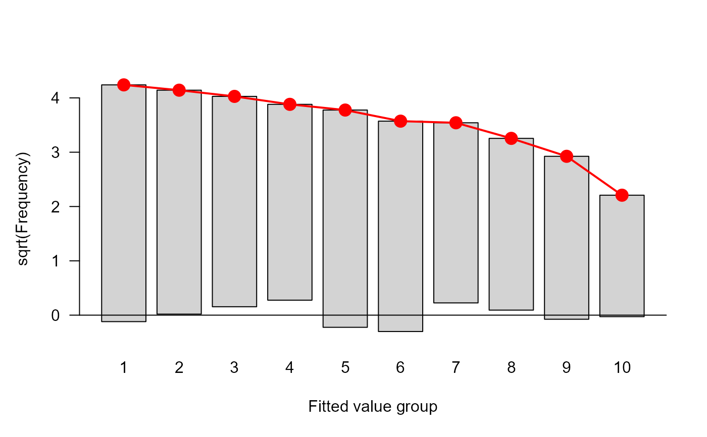
In addition to print and summary methods, a plot method is supplied to visualize the discrepancies between observed and fitted frequencies.

References

Hosmer, David W., Lemeshow, Stanley (1980). A goodness-of-fit test for multiple logistic regression model. Communications in Statistics, Series A, 9, 1043-1069.

Hosmer, David W., Lemeshow, Stanley (2000). Applied Logistic Regression, New York: Wiley, ISBN 0-471-61553-6

Lemeshow, S. and Hosmer, D.W. (1982). A review of goodness of fit statistics for use in the development of logistic regression models. American Journal of Epidemiology, 115(1), 92-106.

Author

Michael Friendly

Examples



data(birthwt, package="MASS")
# how to do this without attach?
attach(birthwt)
#> The following object is masked from package:ca:
#> 
#>     smoke
  race = factor(race, labels = c("white", "black", "other"))
  ptd = factor(ptl > 0)
  ftv = factor(ftv)
  levels(ftv)[-(1:2)] = "2+"
  bwt <- data.frame(low = factor(low), age, lwt, race,
      smoke = (smoke > 0), ptd, ht = (ht > 0), ui = (ui > 0), ftv)
detach(birthwt)

options(contrasts = c("contr.treatment", "contr.poly"))
BWmod <- glm(low ~ ., family=binomial, data=bwt)

(hlt <- HLtest(BWmod))
#> Hosmer and Lemeshow Goodness-of-Fit Test 
#> 
#> Call:
#> glm(formula = low ~ ., family = binomial, data = bwt)
#>  ChiSquare df   P_value
#>   5.981786  8 0.6492722
str(hlt)
#> List of 6
#>  $ table  :'data.frame':	10 obs. of  5 variables:
#>   ..$ cut  : chr [1:10] "[0.0161,0.0788]" "(0.0788,0.119]" "(0.119,0.189]" "(0.189,0.229]" ...
#>   ..$ total: num [1:10] 19 19 19 19 19 18 19 19 19 19
#>   ..$ obs  : num [1:10] 19 17 15 13 16 15 11 10 9 5
#>   ..$ exp  : num [1:10] 18 17.2 16.2 15.1 14.3 ...
#>   ..$ chi  : num [1:10] 0.242 -0.0374 -0.3036 -0.5317 0.4611 ...
#>  $ chisq  : num 5.98
#>  $ df     : num 8
#>  $ p.value: num 0.649
#>  $ groups : num 10
#>  $ call   : language glm(formula = low ~ ., family = binomial, data = bwt)
#>  - attr(*, "class")= chr "HLtest"
summary(hlt)
#> Partition for Hosmer and Lemeshow Goodness-of-Fit Test 
#> 
#>                cut total obs       exp         chi
#> 1  [0.0161,0.0788]    19  19 17.974124  0.24197519
#> 2   (0.0788,0.119]    19  17 17.154854 -0.03738777
#> 3    (0.119,0.189]    19  15 16.222714 -0.30357311
#> 4    (0.189,0.229]    19  13 15.063836 -0.53174994
#> 5    (0.229,0.268]    19  16 14.259007  0.46105470
#> 6    (0.268,0.312]    18  15 12.757257  0.62791490
#> 7    (0.312,0.402]    19  11 12.545096 -0.43623285
#> 8    (0.402,0.493]    19  10 10.593612 -0.18238140
#> 9    (0.493,0.618]    19   9  8.552849  0.15289685
#> 10   (0.618,0.904]    19   5  4.876650  0.05585725
#> Hosmer and Lemeshow Goodness-of-Fit Test 
#> 
#> Call:
#> glm(formula = low ~ ., family = binomial, data = bwt)
#>  ChiSquare df   P_value
#>   5.981786  8 0.6492722
plot(hlt)


# basic model
BWmod0 <- glm(low ~ age, family=binomial, data=bwt)
(hlt0 <- HLtest(BWmod0))
#> Hosmer and Lemeshow Goodness-of-Fit Test 
#> 
#> Call:
#> glm(formula = low ~ age, family = binomial, data = bwt)
#>  ChiSquare df   P_value
#>   9.307311  8 0.3170385
str(hlt0)
#> List of 6
#>  $ table  :'data.frame':	10 obs. of  5 variables:
#>   ..$ cut  : chr [1:10] "[0.128,0.231]" "(0.231,0.26]" "(0.26,0.29]" "(0.29,0.301]" ...
#>   ..$ total: num [1:10] 20 23 26 13 13 25 18 16 22 13
#>   ..$ obs  : num [1:10] 17 19 14 8 8 18 10 13 15 8
#>   ..$ exp  : num [1:10] 15.76 17.23 18.6 9.09 8.95 ...
#>   ..$ chi  : num [1:10] 0.311 0.426 -1.066 -0.361 -0.317 ...
#>  $ chisq  : num 9.31
#>  $ df     : num 8
#>  $ p.value: num 0.317
#>  $ groups : num 10
#>  $ call   : language glm(formula = low ~ age, family = binomial, data = bwt)
#>  - attr(*, "class")= chr "HLtest"
summary(hlt0)
#> Partition for Hosmer and Lemeshow Goodness-of-Fit Test 
#> 
#>              cut total obs       exp         chi
#> 1  [0.128,0.231]    20  17 15.764147  0.31126591
#> 2   (0.231,0.26]    23  19 17.229899  0.42643885
#> 3    (0.26,0.29]    26  14 18.599113 -1.06641920
#> 4   (0.29,0.301]    13   8  9.088499 -0.36106223
#> 5  (0.301,0.312]    13   8  8.947209 -0.31666633
#> 6  (0.312,0.334]    25  18 16.793786  0.29434049
#> 7  (0.334,0.346]    18  10 11.779364 -0.51844629
#> 8  (0.346,0.357]    16  13 10.284015  0.84692725
#> 9  (0.357,0.381]    22  15 13.736398  0.34093679
#> 10 (0.381,0.418]    13   8  7.777571  0.07975704
#> Hosmer and Lemeshow Goodness-of-Fit Test 
#> 
#> Call:
#> glm(formula = low ~ age, family = binomial, data = bwt)
#>  ChiSquare df   P_value
#>   9.307311  8 0.3170385
plot(hlt0)