Minnesota high school graduates of June 1930 were classified with respect to
(a) Rank by thirds in their graduating class, (b) post-high school
Status in April 1939 (4 levels), (c) Sex, (d) father's
Occupational status (7 levels, from 1=High to 7=Low).
Format
A 4-dimensional array resulting from cross-tabulating 4 variables for 13968 observations. The variable names and their levels are:
| No | Name | Levels |
| 1 | Status | "College", "School", "Job", "Other" |
| 2 | Rank | "Low", "Middle", "High" |
| 3 | Occupation | "1", "2", "3", "4", "5", "6", "7" |
| 4 | Sex | "Male", "Female" |
Source
Fienberg, S. E. (1980). The Analysis of Cross-Classified Categorical Data. Cambridge, MA: MIT Press, p. 91-92.
R. L. Plackett, (1974). The Analysis of Categorical Data. London: Griffin.
Details
The data were first presented by Hoyt et al. (1959) and have been analyzed by Fienberg(1980), Plackett(1974) and others.
Post high-school Status is natural to consider as the response.
Rank and father's Occupation are ordinal variables.
References
Hoyt, C. J., Krishnaiah, P. R. and Torrance, E. P. (1959) Analysis of complex contingency tables, Journal of Experimental Education 27, 187-194.
See also
minn38 provides the same data as a data frame.
Examples
data(Hoyt)
# display the table
structable(Status + Sex ~ Rank + Occupation, data=Hoyt)
#> Status College School Job Other
#> Sex Male Female Male Female Male Female Male Female
#> Rank Occupation
#> Low 1 87 53 3 7 17 13 105 76
#> 2 72 36 6 16 18 11 209 111
#> 3 52 52 17 28 14 49 541 521
#> 4 88 48 9 18 14 29 328 191
#> 5 32 12 1 5 12 10 124 101
#> 6 14 9 2 1 5 15 148 130
#> 7 20 3 3 1 4 6 109 88
#> Middle 1 216 163 4 30 14 28 118 118
#> 2 159 116 14 41 28 53 227 214
#> 3 119 162 13 64 44 129 578 708
#> 4 158 130 15 47 36 62 304 305
#> 5 43 35 5 11 7 37 119 152
#> 6 24 19 6 13 15 22 131 174
#> 7 41 25 5 9 13 15 88 158
#> High 1 256 309 2 17 10 38 53 89
#> 2 176 225 8 49 22 68 95 210
#> 3 119 243 10 79 33 184 257 448
#> 4 144 237 12 57 20 63 115 219
#> 5 42 72 2 20 7 21 56 95
#> 6 24 42 2 10 4 19 61 105
#> 7 32 36 2 14 4 19 41 93
# mosaic for independence model
plot(Hoyt, shade=TRUE)
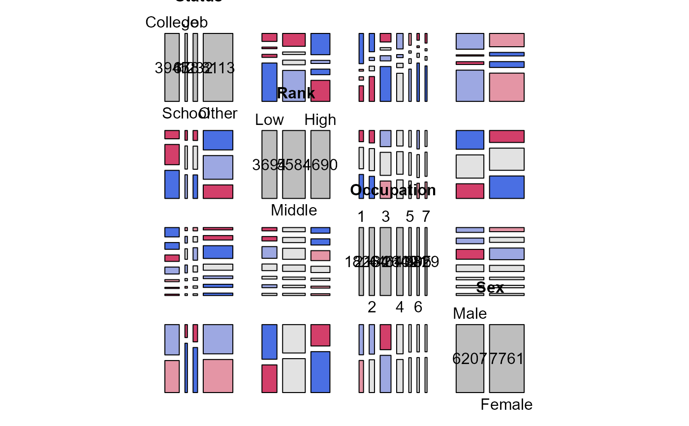
 # examine all pairwise mosaics
pairs(Hoyt, shade=TRUE)
# examine all pairwise mosaics
pairs(Hoyt, shade=TRUE)
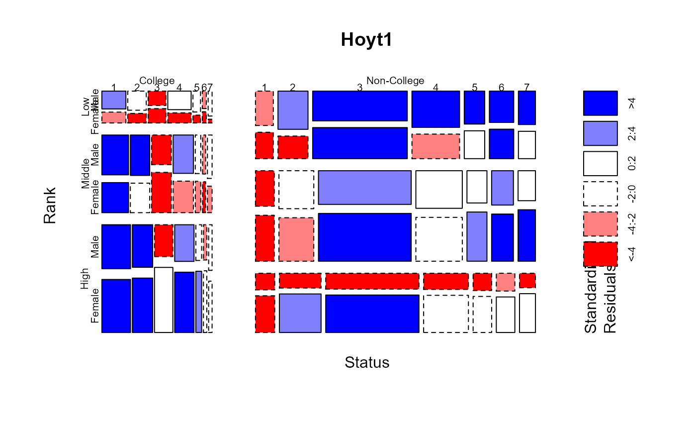
 # collapse Status to College vs. Non-College
Hoyt1 <- collapse.table(Hoyt, Status=c("College", rep("Non-College",3)))
plot(Hoyt1, shade=TRUE)
# collapse Status to College vs. Non-College
Hoyt1 <- collapse.table(Hoyt, Status=c("College", rep("Non-College",3)))
plot(Hoyt1, shade=TRUE)
 #################################################
# fitting models with loglm, plotting with mosaic
#################################################
# fit baseline log-linear model for Status as response
require(MASS)
hoyt.mod0 <- loglm(~ Status + (Sex*Rank*Occupation),
data=Hoyt1)
hoyt.mod0
#> Call:
#> loglm(formula = ~Status + (Sex * Rank * Occupation), data = Hoyt1)
#>
#> Statistics:
#> X^2 df P(> X^2)
#> Likelihood Ratio 2080.359 41 0
#> Pearson 2090.750 41 0
mosaic(hoyt.mod0,
gp=shading_Friendly,
main="Baseline model: Status + (Sex*Rank*Occ)")
#> Error in eval(expr, p): object 'Hoyt1' not found
# add one-way association of Status with factors
hoyt.mod1 <- loglm(~ Status * (Sex + Rank + Occupation) + (Sex*Rank*Occupation),
data=Hoyt1)
hoyt.mod1
#> Call:
#> loglm(formula = ~Status * (Sex + Rank + Occupation) + (Sex *
#> Rank * Occupation), data = Hoyt1)
#>
#> Statistics:
#> X^2 df P(> X^2)
#> Likelihood Ratio 50.10913 32 0.02175915
#> Pearson 49.33936 32 0.02578430
mosaic(hoyt.mod1,
gp=shading_Friendly,
main="Status * (Sex + Rank + Occ)")
#> Error in eval(expr, p): object 'Hoyt1' not found
# can we drop any terms?
drop1(hoyt.mod1, test="Chisq")
#> Error in eval(expr, p): object 'Hoyt1' not found
# assess model fit
anova(hoyt.mod0, hoyt.mod1)
#> LR tests for hierarchical log-linear models
#>
#> Model 1:
#> ~Status + (Sex * Rank * Occupation)
#> Model 2:
#> ~Status * (Sex + Rank + Occupation) + (Sex * Rank * Occupation)
#>
#> Deviance df Delta(Dev) Delta(df) P(> Delta(Dev)
#> Model 1 2080.35910 41
#> Model 2 50.10913 32 2030.24997 9 0.00000
#> Saturated 0.00000 0 50.10913 32 0.02176
# what terms to add?
add1(hoyt.mod1, ~.^2, test="Chisq")
#> Error in eval(expr, p): object 'Hoyt1' not found
# add interaction of Sex:Occupation on Status
hoyt.mod2 <- update(hoyt.mod1, ~ . + Status:Sex:Occupation)
mosaic(hoyt.mod2,
gp=shading_Friendly,
main="Adding Status:Sex:Occupation")
#> Error in eval(expr, p): object 'Hoyt1' not found
# compare model fits
anova(hoyt.mod0, hoyt.mod1, hoyt.mod2)
#> LR tests for hierarchical log-linear models
#>
#> Model 1:
#> ~Status + (Sex * Rank * Occupation)
#> Model 2:
#> ~Status * (Sex + Rank + Occupation) + (Sex * Rank * Occupation)
#> Model 3:
#> ~Status + Sex + Rank + Occupation + Status:Sex + Status:Rank + Status:Occupation + Sex:Rank + Sex:Occupation + Rank:Occupation + Sex:Rank:Occupation + Status:Sex:Occupation
#>
#> Deviance df Delta(Dev) Delta(df) P(> Delta(Dev)
#> Model 1 2080.35910 41
#> Model 2 50.10913 32 2030.24997 9 0.00000
#> Model 3 21.01300 26 29.09613 6 0.00006
#> Saturated 0.00000 0 21.01300 26 0.74129
# Alternatively, try stepwise analysis, heading toward the saturated model
steps <- step(hoyt.mod0,
direction="forward",
scope=~Status*Sex*Rank*Occupation)
#> Start: AIC=2166.36
#> ~Status + (Sex * Rank * Occupation)
#>
#> Error in eval(expr, p): object 'Hoyt1' not found
# display anova
steps$anova
#> Error: object 'steps' not found
#################################################
# fitting models with loglm, plotting with mosaic
#################################################
# fit baseline log-linear model for Status as response
require(MASS)
hoyt.mod0 <- loglm(~ Status + (Sex*Rank*Occupation),
data=Hoyt1)
hoyt.mod0
#> Call:
#> loglm(formula = ~Status + (Sex * Rank * Occupation), data = Hoyt1)
#>
#> Statistics:
#> X^2 df P(> X^2)
#> Likelihood Ratio 2080.359 41 0
#> Pearson 2090.750 41 0
mosaic(hoyt.mod0,
gp=shading_Friendly,
main="Baseline model: Status + (Sex*Rank*Occ)")
#> Error in eval(expr, p): object 'Hoyt1' not found
# add one-way association of Status with factors
hoyt.mod1 <- loglm(~ Status * (Sex + Rank + Occupation) + (Sex*Rank*Occupation),
data=Hoyt1)
hoyt.mod1
#> Call:
#> loglm(formula = ~Status * (Sex + Rank + Occupation) + (Sex *
#> Rank * Occupation), data = Hoyt1)
#>
#> Statistics:
#> X^2 df P(> X^2)
#> Likelihood Ratio 50.10913 32 0.02175915
#> Pearson 49.33936 32 0.02578430
mosaic(hoyt.mod1,
gp=shading_Friendly,
main="Status * (Sex + Rank + Occ)")
#> Error in eval(expr, p): object 'Hoyt1' not found
# can we drop any terms?
drop1(hoyt.mod1, test="Chisq")
#> Error in eval(expr, p): object 'Hoyt1' not found
# assess model fit
anova(hoyt.mod0, hoyt.mod1)
#> LR tests for hierarchical log-linear models
#>
#> Model 1:
#> ~Status + (Sex * Rank * Occupation)
#> Model 2:
#> ~Status * (Sex + Rank + Occupation) + (Sex * Rank * Occupation)
#>
#> Deviance df Delta(Dev) Delta(df) P(> Delta(Dev)
#> Model 1 2080.35910 41
#> Model 2 50.10913 32 2030.24997 9 0.00000
#> Saturated 0.00000 0 50.10913 32 0.02176
# what terms to add?
add1(hoyt.mod1, ~.^2, test="Chisq")
#> Error in eval(expr, p): object 'Hoyt1' not found
# add interaction of Sex:Occupation on Status
hoyt.mod2 <- update(hoyt.mod1, ~ . + Status:Sex:Occupation)
mosaic(hoyt.mod2,
gp=shading_Friendly,
main="Adding Status:Sex:Occupation")
#> Error in eval(expr, p): object 'Hoyt1' not found
# compare model fits
anova(hoyt.mod0, hoyt.mod1, hoyt.mod2)
#> LR tests for hierarchical log-linear models
#>
#> Model 1:
#> ~Status + (Sex * Rank * Occupation)
#> Model 2:
#> ~Status * (Sex + Rank + Occupation) + (Sex * Rank * Occupation)
#> Model 3:
#> ~Status + Sex + Rank + Occupation + Status:Sex + Status:Rank + Status:Occupation + Sex:Rank + Sex:Occupation + Rank:Occupation + Sex:Rank:Occupation + Status:Sex:Occupation
#>
#> Deviance df Delta(Dev) Delta(df) P(> Delta(Dev)
#> Model 1 2080.35910 41
#> Model 2 50.10913 32 2030.24997 9 0.00000
#> Model 3 21.01300 26 29.09613 6 0.00006
#> Saturated 0.00000 0 21.01300 26 0.74129
# Alternatively, try stepwise analysis, heading toward the saturated model
steps <- step(hoyt.mod0,
direction="forward",
scope=~Status*Sex*Rank*Occupation)
#> Start: AIC=2166.36
#> ~Status + (Sex * Rank * Occupation)
#>
#> Error in eval(expr, p): object 'Hoyt1' not found
# display anova
steps$anova
#> Error: object 'steps' not found