Mental Impairment and Parents SES

A 6 x 4 contingency table representing the cross-classification of mental health status (mental) of 1660 young New York residents by their parents' socioeconomic status (ses).

Usage

data(Mental)

Format

A data frame frequency table with 24 observations on the following 3 variables.

ses

an ordered factor with levels 1 < 2 < 3 < 4 < 5 < 6

mental

an ordered factor with levels Well < Mild < Moderate < Impaired

Freq

cell frequency: a numeric vector

Details

Both ses and mental can be treated as ordered factors or integer scores. For ses, 1="High" and 6="Low".

Source

Haberman, S. J. The Analysis of Qualitative Data: New Developments, Academic Press, 1979, Vol. II, p. 375.

Srole, L.; Langner, T. S.; Michael, S. T.; Kirkpatrick, P.; Opler, M. K. & Rennie, T. A. C. Mental Health in the Metropolis: The Midtown Manhattan Study, NYU Press, 1978, p. 289

References

Friendly, M. Visualizing Categorical Data, Cary, NC: SAS Institute, 2000, Appendix B.7.

Examples

data(Mental)
str(Mental)
#> 'data.frame':	24 obs. of  3 variables:
#>  $ ses   : Ord.factor w/ 6 levels "1"<"2"<"3"<"4"<..: 1 1 1 1 2 2 2 2 3 3 ...
#>  $ mental: Ord.factor w/ 4 levels "Well"<"Mild"<..: 1 2 3 4 1 2 3 4 1 2 ...
#>  $ Freq  : int  64 94 58 46 57 94 54 40 57 105 ...
(Mental.tab <- xtabs(Freq ~ ses + mental, data=Mental))
#>    mental
#> ses Well Mild Moderate Impaired
#>   1   64   94       58       46
#>   2   57   94       54       40
#>   3   57  105       65       60
#>   4   72  141       77       94
#>   5   36   97       54       78
#>   6   21   71       54       71

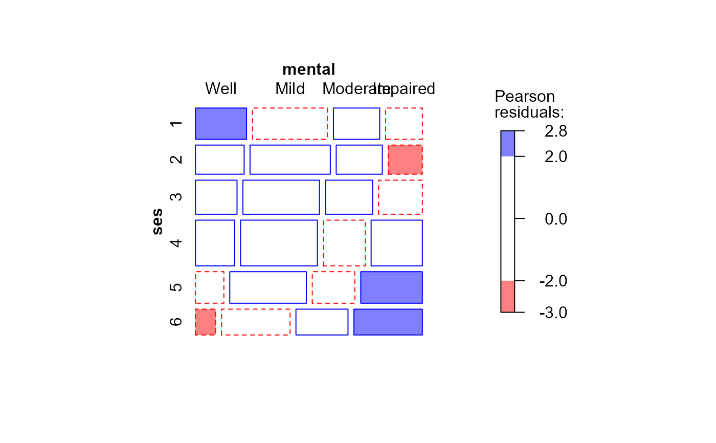
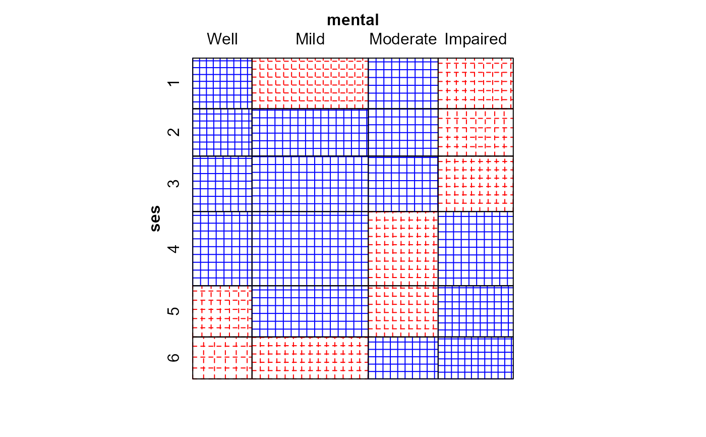
# mosaic and sieve plots
mosaic(Mental.tab, gp=shading_Friendly)

sieve(Mental.tab, gp=shading_Friendly)


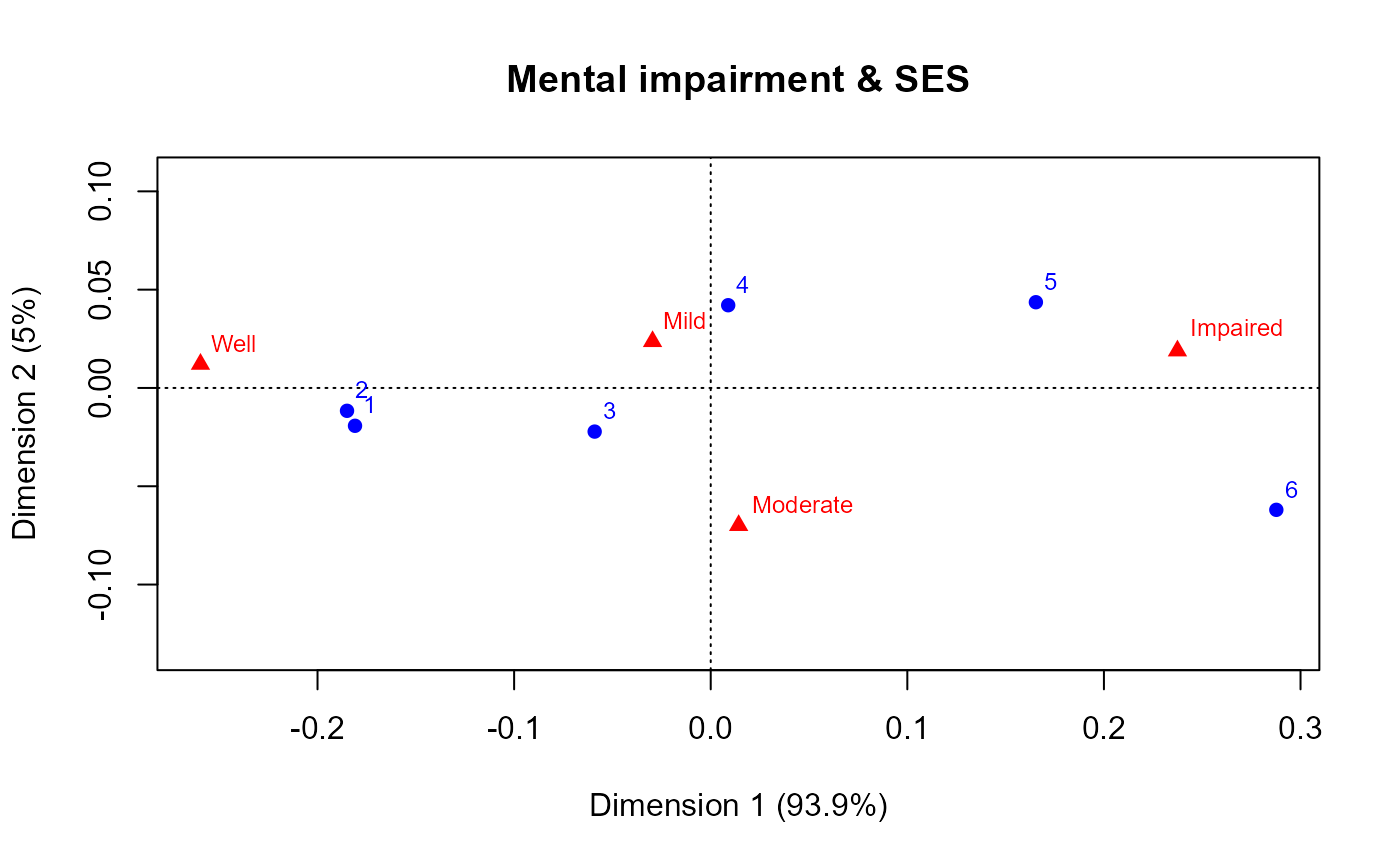
if(require(ca)){
  plot(ca(Mental.tab), main="Mental impairment & SES")
}