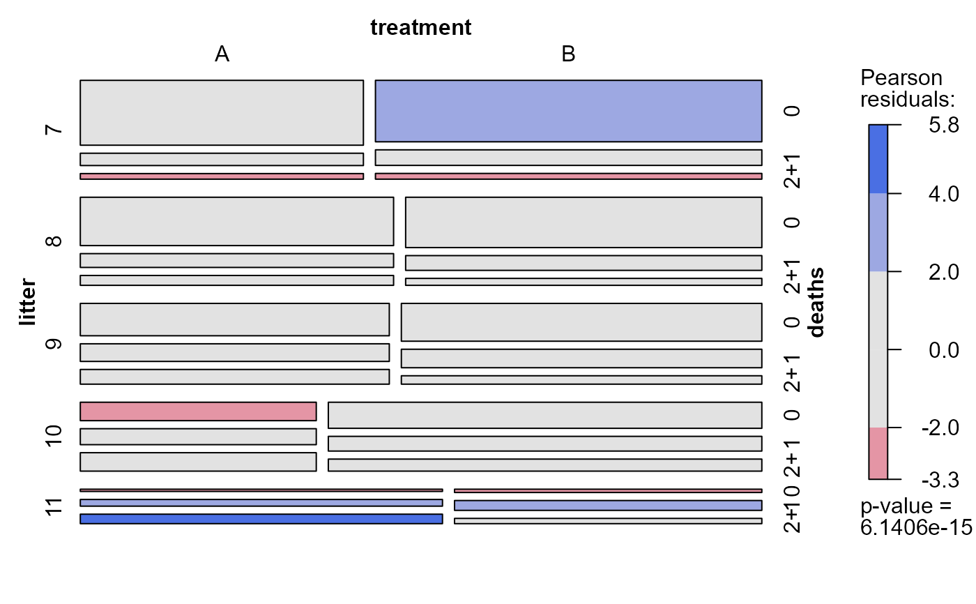
Data from Kastenbaum and Lamphiear (1959). The table gives the number of depletions (deaths) in 657 litters of mice, classified by litter size and treatment. This data set has become a classic in the analysis of contingency tables, yet unfortunately little information on the details of the experiment has been published.
Format
A frequency data frame with 30 observations on the following 4 variables, representing a 5 x 2 x 3 contingency table.
litterlitter size, a numeric vector
treatmenttreatment, a factor with levels
ABdeathsnumber of depletions, a factor with levels
012+Freqcell frequency, a numeric vector
Source
Goodman, L. A. (1983) The analysis of dependence in cross-classifications having ordered categories, using log-linear models for frequencies and log-linear models for odds. Biometrics, 39, 149-160.
References
Kastenbaum, M. A. & Lamphiear, D. E. (1959) Calculation of chi-square to calculate the no three-factor interaction hypothesis. Biometrics, 15, 107-115.
Examples
data(Mice)
# make a table
ftable(mice.tab <- xtabs(Freq ~ litter + treatment + deaths, data=Mice))
#>                  deaths  0  1 2+
#> litter treatment
#> 7      A                58 11  5
#>        B                75 19  7
#> 8      A                49 14 10
#>        B                58 17  8
#> 9      A                33 18 15
#>        B                45 22 10
#> 10     A                15 13 15
#>        B                39 22 18
#> 11     A                 4 12 17
#>        B                 5 15  8

#library(vcd)
vcd::mosaic(mice.tab, shade=TRUE)