Plot a fitted logistic regression with marginal distributions of the predictor

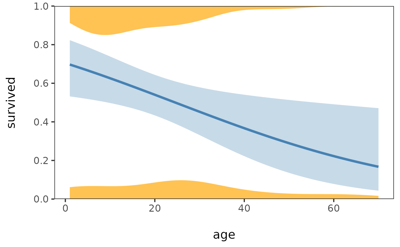
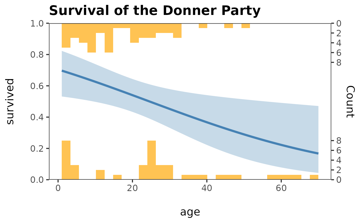
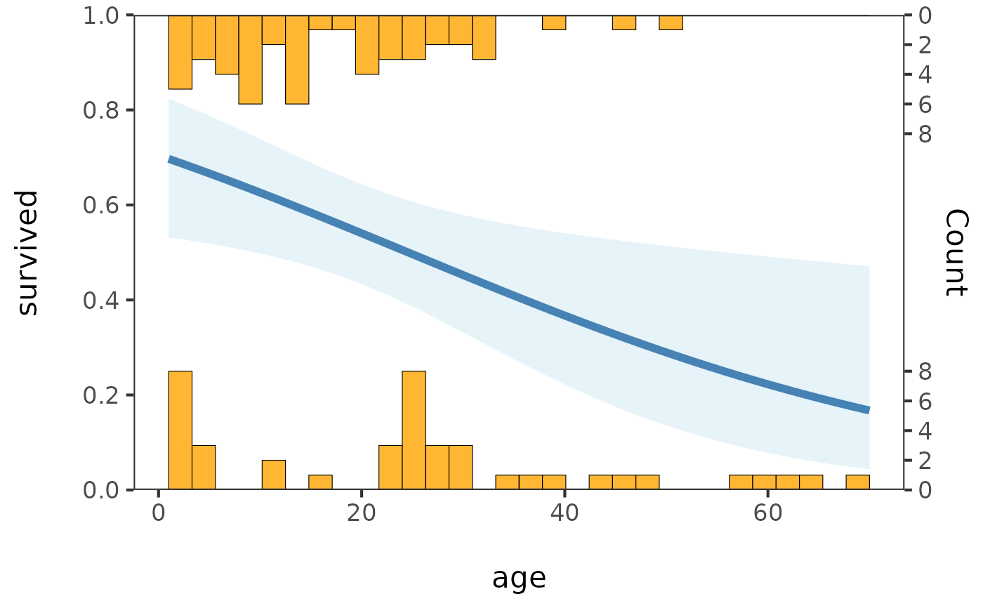
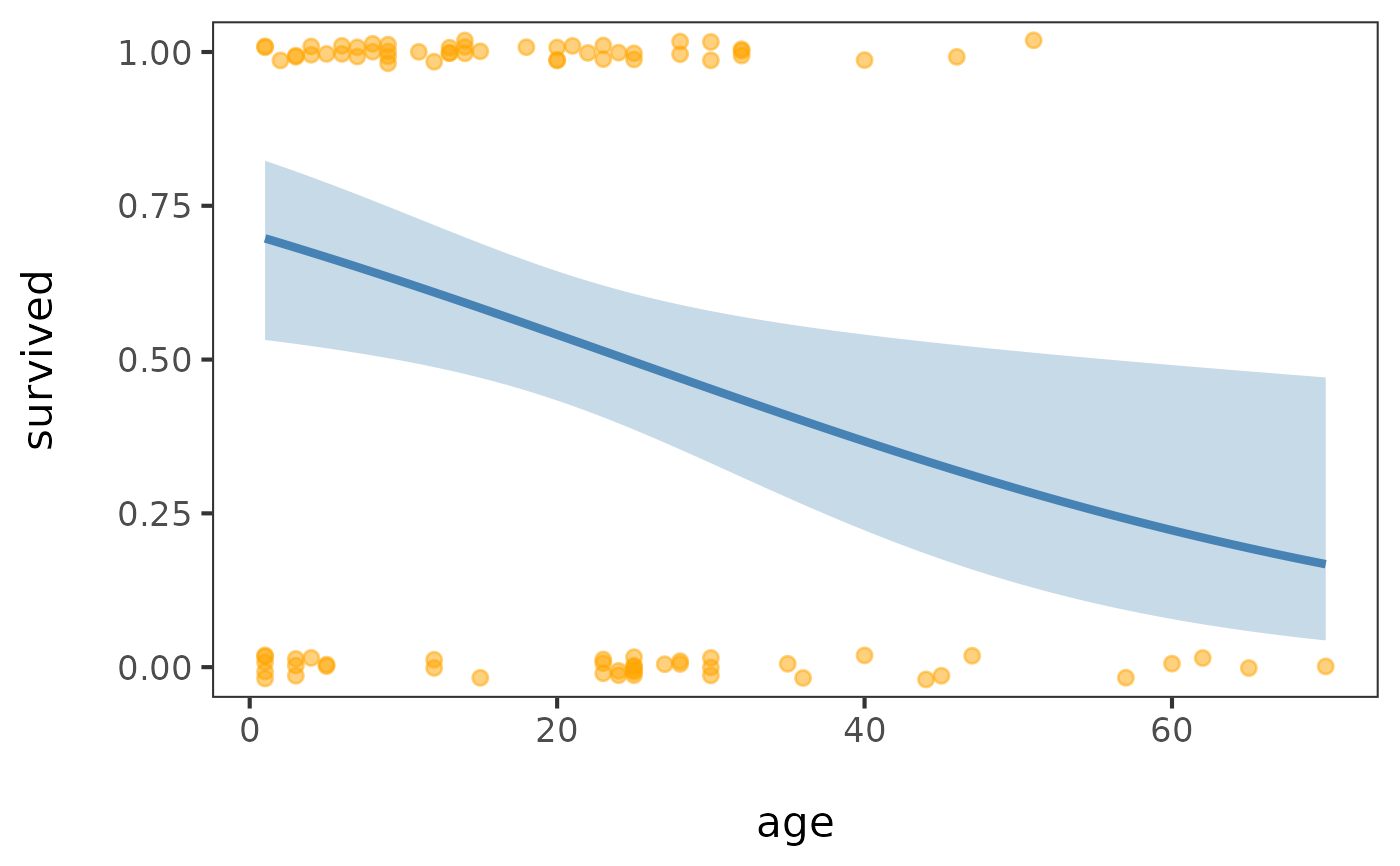
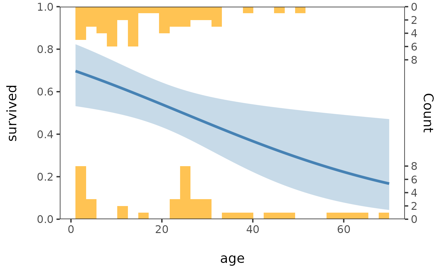
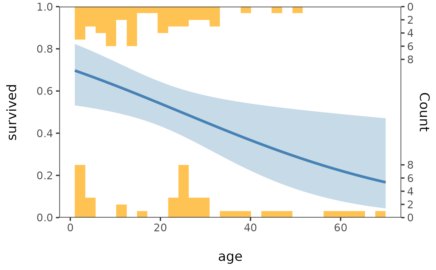
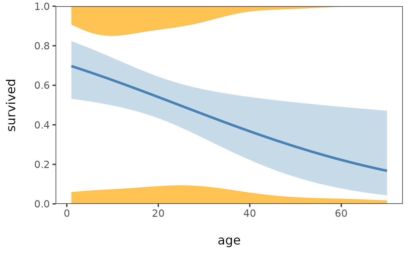
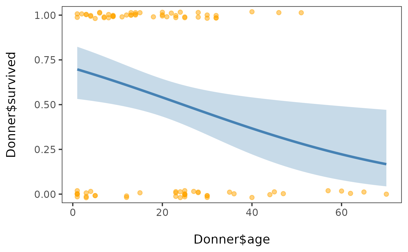
Plots predicted probabilities from a glm(y ~ x, family = binomial) fit for a single quantitative predictor x and binary response y, and also with the smoothed logistic fit and its confidence band. What this plot method adds is a representation of the marginal distribution of x within each y group – mirrored histograms or filled density estimates above and below the curve, or jittered points – as suggested by Smart et al. (2004). These help you see where the data supporting the fit exist; e.g., where the data are "thin", so the confidence band is wide.

Usage

logist_plot(x, ...)

# Default S3 method
logist_plot(
  x,
  y,
  marginal = c("hist", "points", "density"),
  bins = 30,
  adjust = 1,
  xlab = NULL,
  ylab = NULL,
  fit.color = "steelblue",
  marginal.color = "orange",
  fit.args = list(),
  marginal.args = list(),
  group = NULL,
  group.colors = NULL,
  marginal.height = NULL,
  ...
)

# S3 method for class 'data.frame'
logist_plot(
  x,
  xvar = 1L,
  yvar = 2L,
  marginal = c("hist", "points", "density"),
  bins = 30,
  adjust = 1,
  xlab = NULL,
  ylab = NULL,
  fit.color = "steelblue",
  marginal.color = "orange",
  fit.args = list(),
  marginal.args = list(),
  group = NULL,
  group.colors = NULL,
  marginal.height = NULL,
  ...
)

# S3 method for class 'formula'
logist_plot(
  formula,
  data,
  marginal = c("hist", "points", "density"),
  bins = 30,
  adjust = 1,
  xlab = NULL,
  ylab = NULL,
  fit.color = "steelblue",
  marginal.color = "orange",
  fit.args = list(),
  marginal.args = list(),
  group = NULL,
  group.colors = NULL,
  marginal.height = NULL,
  ...
)

logist_hist(...)

logist_point(...)

logist_density(...)

Arguments

x: a numeric predictor vector or a data frame; see formula below for the model-formula interface
...: arguments passed to methods, or on to logist_plot() from the convenience wrappers. Arguments not consumed by the selected method are an error rather than being silently ignored. Use fit.args and marginal.args for layer customization.
y: a binary (0/1, or 2-level factor/character/logical) response vector
marginal: character string, how to represent the marginal distribution of x within each y group: "hist", mirrored histograms (default); "points", jittered points; or "density", mirrored filled density estimates
bins: number of histogram bins, for marginal = "hist"; default: 30
adjust: positive numeric bandwidth adjustment passed to stats::density() for marginal = "density"; default: 1
xlab, ylab: axis labels; default to the deparsed x/y expressions
fit.color: color of the fitted logistic curve and its confidence band; default: "steelblue". This scalar is inactive when group is supplied; use group.colors instead.
marginal.color: color of the marginal representation of x within each y group (histogram/density fill, or point color for marginal = "points"); default: "orange" This scalar is inactive when group is supplied; use group.colors instead.
fit.args: named list of graphical arguments for the fitted curve and confidence band. Values override the defaults established by fit.color. The fit remains a binomial GLM, so data, mapping, stat, position, inherit.aes, method, formula, and method.args cannot be replaced. In grouped mode, colour and fill must instead be controlled through group.colors.
marginal.args: named list of graphical arguments for the active marginal layer. Values override the defaults established by marginal.color. Valid arguments depend on marginal: point aesthetics and position for "points", rectangle aesthetics for "hist", or ribbon aesthetics for "density". Histogram computation remains controlled by bins; density bandwidth remains controlled by adjust; and marginal geometry height remains controlled by marginal.height. In grouped mode, colour and fill must instead be controlled through group.colors.
group: optional grouping input. For the default method, a vector the same length as x and y; for data-frame and formula methods, a single column name or position. Grouping is supported for marginal = "points" and "density", but not "hist".
group.colors: optional character vector of colours for grouped plots. An unnamed vector is applied in group-level order; a named vector must contain every observed group label. The same palette is used for fits, marginals, and the legend. The default NULL uses ggplot2's discrete scales.
marginal.height: optional finite positive number controlling marginal height. For histograms and ungrouped densities, this is the maximum proportion of the fixed 0–1 probability panel occupied on each side; defaults are 0.25 and 0.15, respectively, and values cannot exceed 0.5. For grouped densities, it is the full height of each outward lane in the original probability-coordinate units; the default is 0.05 and values cannot exceed 1. NULL selects the applicable default. For marginal = "points", a non-NULL value is ignored with a warning; control vertical jitter through marginal.args instead.
xvar, yvar: which columns of x to use as predictor/response – column name or position; default to the first two columns (matches the original 2-column-data-frame calling convention)
formula: a model formula, y ~ x – exactly one response and one predictor; formula method only. The first argument may be passed positionally or as formula = y ~ x (matching base R's boxplot()/lm() convention) – unlike the other methods, it is not named x
data: a data frame – formula method only

Value

A native ggplot object that can be extended with ordinary ggplot2 additions.

Details

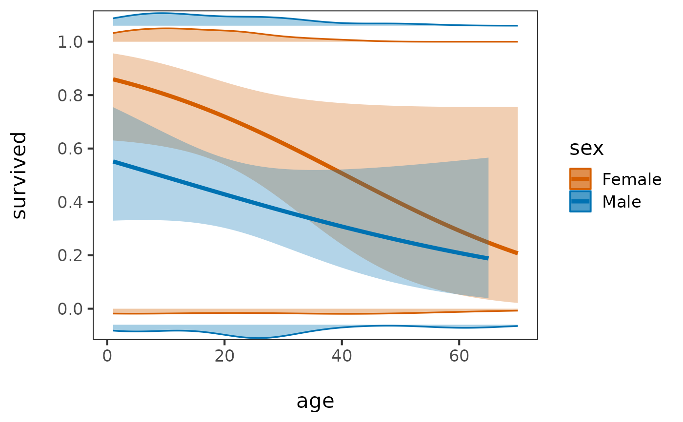
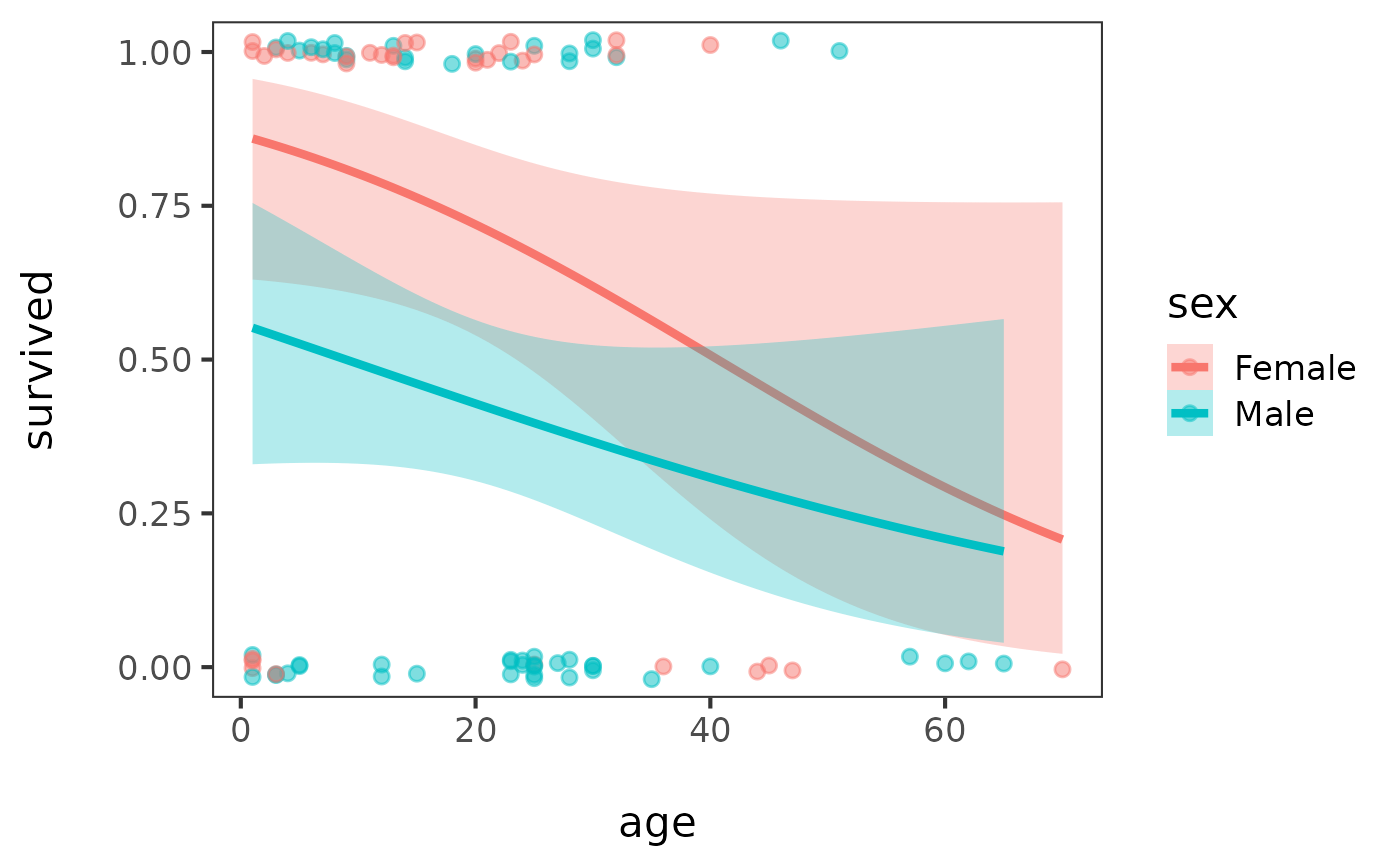
logist_plot() is generic, with methods for a pair of vectors, a data frame, or a model formula. logist_hist(), logist_point(), and logist_density() are convenience wrappers with marginal= fixed to "hist"/"points"/"density", but otherwise accept the same x/... as logist_plot() – i.e., they also work with a data frame or a formula. An optional group produces separate fits and colour identities in point and density modes. Grouped histograms are deliberately unsupported because stacked or overlapping mirrored bars obscure both the distributions and the fitted curves. Grouped density lanes begin at 0 and 1 and stack outward in fixed, narrow bands. Each group's two response-specific densities are normalized together within that band, so the shapes show conditional distributions but do not encode group sample sizes.

bins, adjust, and marginal.height control computation of the marginal geometry; they are not graphical layer arguments and therefore belong at the top level rather than inside marginal.args. When a small histogram height would crowd the secondary count axis, its integer ticks are thinned symmetrically while retaining the correct count-to-height mapping.

All marginal modes return a native ggplot object. Standard additions such as ggplot2::labs() and ggplot2::theme() can therefore be applied after construction. Adding another scale_y_*() replaces the internally configured probability scale; in histogram mode this can remove or invalidate the secondary count-axis mapping.

References

Smart, J. M. R., Sutherland, W. J., Watkinson, A. R., and Gill, J. A. (2004). A New Means of Presenting the Results of Logistic Regression, Bulletin of the Ecological Society of America, 85(3), 100–102. doi:10.1890/0012-9623(2004)85[100:ANMOPT]2.0.CO;2 https://esapubs.org/bulletin/backissues/085-3/bulletinjuly2004_2column.htm#tools1

Author

Gavin Klorfine, Michael Friendly

Examples

data(Donner, package = "vcdExtra")

# three interfaces to the same underlying plot
logist_plot(Donner$age, Donner$survived, marginal = "points")

logist_plot(Donner[, c("age", "survived")], marginal = "hist")

logist_plot(survived ~ age, data = Donner, marginal = "density")


# post-hoc labels and themes work in histogram mode
logist_plot(survived ~ age, data = Donner, marginal = "hist") +
  ggplot2::labs(title = "Survival of the Donner Party") +
  ggplot2::theme(plot.title = ggplot2::element_text(face = "bold"))


# layer-specific customization; scoped lists override graphical defaults
logist_plot(
  survived ~ age, data = Donner, marginal = "hist",
  fit.args = list(linewidth = 2, fill = "lightblue"),
  marginal.args = list(colour = "black", linewidth = 0.2, alpha = 0.8)
)


# convenience wrappers -- marginal= fixed, still get all calling conventions
logist_point(survived ~ age, data = Donner)

logist_hist(survived ~ age, data = Donner)

logist_density(survived ~ age, data = Donner, adjust = 1.25)


# grouped fits and marginals; grouped density lanes extend outward from 0 and 1
logist_point(survived ~ age, data = Donner, group = "sex")

logist_density(
  survived ~ age, data = Donner, group = "sex",
  group.colors = c(Female = "#D55E00", Male = "#0072B2"),
  marginal.args = list(alpha = 0.35, linewidth = 0.6)
)