Reading and Arithmetic Achievement in Children with Learning Disabilities

A small factorial dataset from Tabachnick & Fidell (2013) relating a treatment/control intervention and degree of disability to reading and arithmetic achievement test scores, with IQ also recorded. It is not clear whether this is fictitious data or derived from a real study.

It provides for simple examples of MANOVA, MANCOVA and stepdown analysis

Usage

data("LearnDis")

Format

A data frame with 18 observations on the following 5 variables, a 3 (Disability) x 2 (Treatment) between-subjects factorial with n = 3 per cell.

Disability: Degree of disability, an ordered factor with levels Mild < Moderate < Severe
Treatment: a factor with levels Treatment Control
WRAT_R: Wide Range Achievement Test, Reading subtest score, a numeric vector
WRAT_A: Wide Range Achievement Test, Arithmetic subtest score, a numeric vector
IQ: IQ score, a numeric vector – used in the source as a MANCOVA covariate, not part of the stepdown analysis itself

Source

Tabachnick, B. G., & Fidell, L. S. (2013). Using Multivariate Statistics (6th ed.). Pearson. Table 7.1, p.256.

References

The Roy-Bargmann stepdown analysis of this data (WRAT-R prioritized over WRAT-A) appears in the same source, §7.5.3.2, Tables 7.7-7.9, pp.273-274.

Roy, S. N. (1958). Step-Down Procedure in Multivariate Analysis. The Annals of Mathematical Statistics, 29(4), 1177-1187. doi:10.1214/aoms/1177706449 .

Examples

data(LearnDis)
str(LearnDis)
#> 'data.frame':	18 obs. of  5 variables:
#>  $ Disability: Ord.factor w/ 3 levels "Mild"<"Moderate"<..: 1 1 1 2 2 2 3 3 3 1 ...
#>  $ Treatment : Factor w/ 2 levels "Treatment","Control": 1 1 1 1 1 1 1 1 1 2 ...
#>  $ WRAT_R    : num  115 98 107 100 105 95 89 100 90 90 ...
#>  $ WRAT_A    : num  108 105 98 105 95 98 78 85 95 92 ...
#>  $ IQ        : num  110 102 100 115 98 100 99 102 100 108 ...

ld.mod <- lm(cbind(WRAT_R, WRAT_A) ~ Disability * Treatment, data = LearnDis)
car::Anova(ld.mod)
#> 
#> Type II MANOVA Tests: Pillai test statistic
#>                      Df test stat approx F num Df den Df    Pr(>F)    
#> Disability            2   0.75048    3.604      4     24   0.01946 *  
#> Treatment             1   0.86228   34.436      2     11 1.839e-05 ***
#> Disability:Treatment  2   0.09219    0.290      4     24   0.88160    
#> ---
#> Signif. codes:  0 '***' 0.001 '**' 0.01 '*' 0.05 '.' 0.1 ' ' 1

heplot(ld.mod, fill = TRUE, fill.alpha = 0.1)


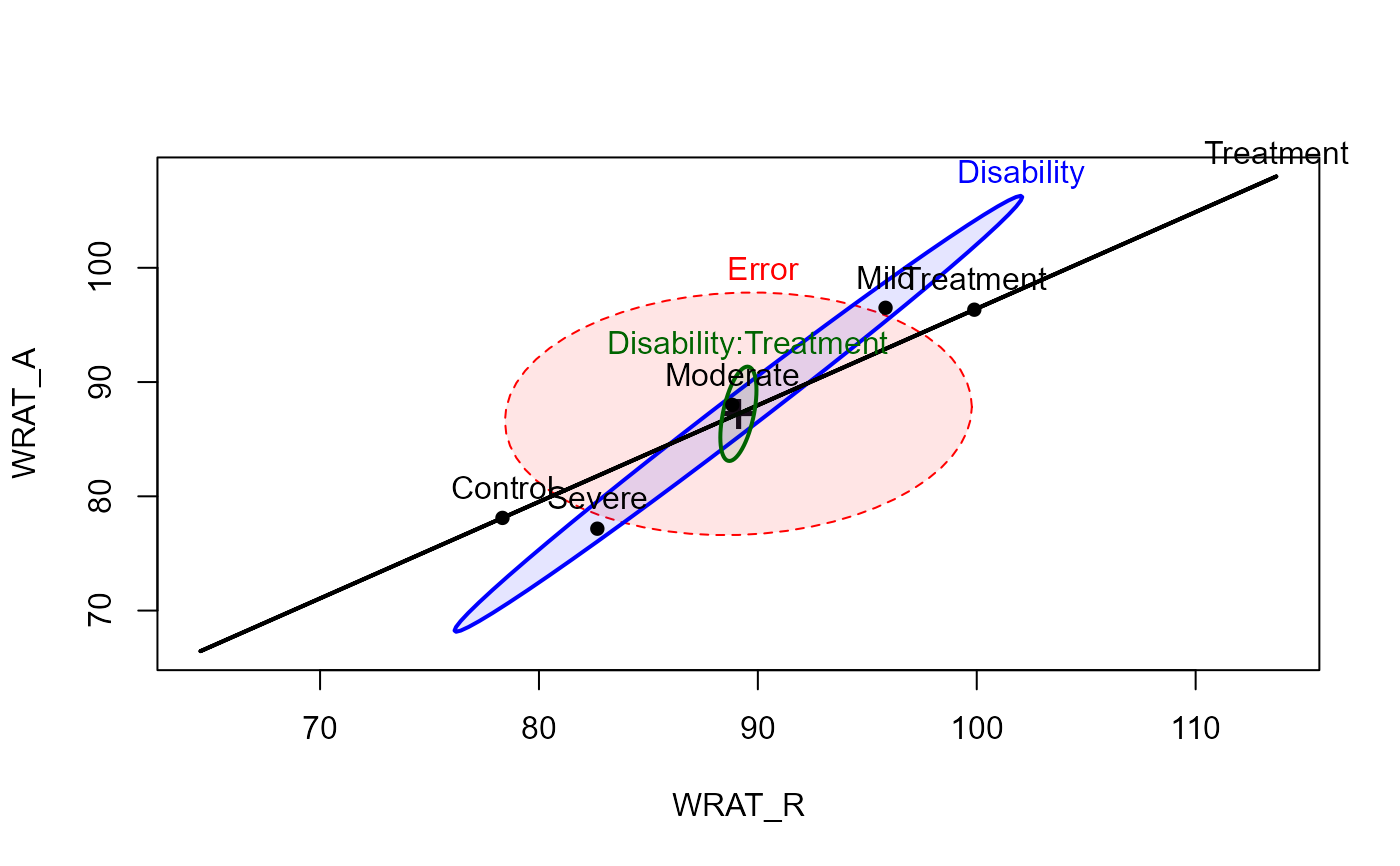# Roy-Bargmann stepdown: does WRAT-A add anything to WRAT-R for the
# Treatment effect? 
# Needs Type III SS, since the WRAT_R covariate breaks the balanced
# factorial's orthogonality:
options(contrasts = c("contr.sum", "contr.poly"))
step2.mod <- lm(WRAT_A ~ WRAT_R + Disability * Treatment, data = LearnDis)
car::Anova(step2.mod, type = "III")
#> Anova Table (Type III tests)
#> 
#> Response: WRAT_A
#>                      Sum Sq Df F value  Pr(>F)  
#> (Intercept)          460.51  1  9.4232 0.01067 *
#> WRAT_R                 1.77  1  0.0361 0.85267  
#> Disability           538.37  2  5.5082 0.02201 *
#> Treatment            268.31  1  5.4903 0.03896 *
#> Disability:Treatment  52.13  2  0.5334 0.60104  
#> Residuals            537.57 11                  
#> ---
#> Signif. codes:  0 '***' 0.001 '**' 0.01 '*' 0.05 '.' 0.1 ' ' 1