Robust Multivariate Linear Models

Abstract

This vignette describes the theory behind, and demonstrates the use of, the robmlm() function from the heplots package, which provides robust estimation for multivariate linear models (MLMs) using iteratively reweighted least squares (IRLS).

It illustrates the central ideas behind robust estimation for MLMs, how the IRLS algorithm works, and presents examples of plots that help understand how robust models can contribute to data analysis.

Load packages

I use the following packages here:

library(heplots)
library(candisc)
library(ggplot2)
library(dplyr)
library(mvinfluence)

Introduction

Multivariate linear models (MLMs) extend the familiar univariate linear regression framework to situations where multiple response variables are modeled simultaneously as linear functions of a common set of predictor variables. While classical multivariate least squares estimation provides optimal results under ideal conditions (multivariate normality and absence of outliers), real-world data often violate these assumptions. The presence of outliers, heavy-tailed distributions, or other departures from normality can severely compromise the reliability of classical estimators, leading to biased parameter estimates and inflated error rates in hypothesis testing.

The need for robust estimation in multivariate regression has been recognized since the early development of robust statistical methods (Huber, 1964; Tukey, 1960). Outliers in multivariate data can be particularly problematic because they may not be readily apparent when examining univariate marginal distributions, yet can exert substantial leverage on the fitted model. Furthermore, the curse of dimensionality means that as the number of response variables increases, the probability of encountering at least one outlying observation grows rapidly.

Robust multivariate regression methods aim to provide reliable parameter estimates and inference procedures that remain stable in the presence of outlying observations. As noted by Rousseeuw, Van Aelst, Van Driessen, & Gulló (2004), “The main advantage of robust regression is that it provides reliable results even when some of the assumptions of classical regression are violated.”

Several approaches have been developed for robust multivariate regression, including M-estimators, S-estimators (Rousseeuw & Yohai, 1984), and MM-estimators (Yohai, 1987). Each approach offers different trade-offs between robustness properties, computational efficiency, and statistical efficiency under ideal conditions. See the CRAN Task View: Robust Statistical Methods for an extensive list of robust methods in R and the vignette for the rrcov package for a general overview of multivariate robust methods.

The method implemented in the robmlm() function belongs to the class of M-estimators, which generalize maximum likelihood estimation by replacing the likelihood function with a more robust objective function.

The key idea is to relax the least squares criterion of minimizing $Q(\mathbf{e}) = \Sigma e_i^2 = \Sigma (y_i - \hat{y}_i)^2$ by considering more general functions $Q(\mathbf{e}, \rho)$ , where the function $\rho (e_i)$ can be chosen to reduce the impact of large outliers. In these terms,

OLS uses $\rho(e_i) = e_i^2$
$L_1$ estimation uses $\rho(e_i) = \vert e_i \vert$ , the least absolute values
A bit more complicated, the biweight function uses a squared measure of error up to some value $c$ and then levels off thereafter,

$\rho(e_i) = \begin{cases} \left[ 1 - \left( \frac{e_i}{c} \right)^2 \right]^2 & |e_i| \leq c, \\ 1 & |e_i| > c. \end{cases}$

These functions look like this in a graph. For the biweight function has a property like Windsorizing— the squared error remains constant for residuals $e_i > c$ , with $c = 4.685$ for MASS::psi.bisquare().

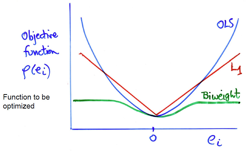
$Diagram ploting the function $\rho(e_i)$ of the contributions of the residuals $e_i$ to what is minimized in various fitting methods.$

Figure 1: Diagram ploting the function $\rho(e_i)$ of the contributions of the residuals $e_i$ to what is minimized in various fitting methods.

Methodology: Iteratively Reweighted Least Squares (IRLS)

The robmlm() function implements robust multivariate linear model fitting using Iteratively Reweighted Least Squares (IRLS), a flexible and computationally efficient approach that belongs to the family of M-estimators. The core idea behind IRLS is to iteratively downweight observations that appear to be outliers based on their residual distances from the fitted model.

The IRLS Algorithm

The IRLS algorithm for robust multivariate regression is shown in the figure below.

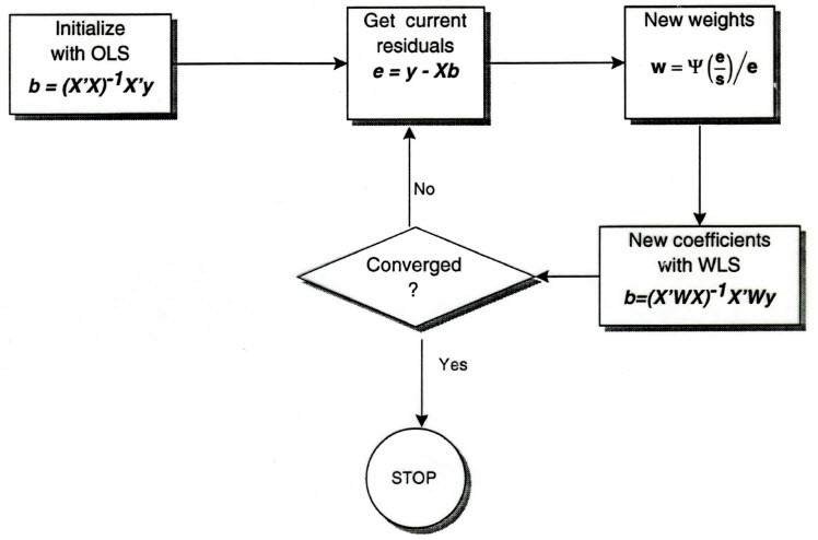
Figure 2: Flowchart for the iteratively reweighted least squares algorithm

The method proceeds as follows:

Initialization: Begin with an initial estimate of the regression coefficients, typically obtained from ordinary least squares (OLS).
Residual calculation: Compute the multivariate residuals for each observation: $\mathbf{r}_i = \mathbf{y}_i - \mathbf{X}_i\hat{\boldsymbol{\beta}}$ where $\mathbf{y}_i$ is the $p \times 1$ response vector for observation $i$ , $\mathbf{X}_i$ is the corresponding row of the design matrix, and $\hat{\boldsymbol{\beta}}$ is the current estimate of the coefficient matrix.
Distance computation: Calculate the squared Mahalanobis distance of each residual vector from the origin: $d_i^2 = \mathbf{r}_i^T \mathbf{S}^{-1} \mathbf{r}_i$ where $\mathbf{S}$ is a robust estimate of the residual covariance matrix, computed using MASS::cov.trob().
Weight assignment: Assign weights to each observation based on their residual distances. Observations with larger distances receive smaller weights, effectively downweighting potential outliers: $w_i = \rho(d_i^2)$ where $\rho(\cdot)$ is a weight function that decreases as the distance increases.
Weighted Least Squares: Update the coefficient estimates using weighted least squares: $\hat{\boldsymbol{\beta}}^{(new)} = (\mathbf{X}^T\mathbf{W}\mathbf{X})^{-1}\mathbf{X}^T\mathbf{W}\mathbf{Y}$ where $\mathbf{W}$ is a diagonal matrix of weights.
Convergence check: Repeat steps 2-5 until convergence, typically assessed by monitoring changes in the coefficient estimates or weights between iterations.

Features of the Implementation

The robmlm() implementation incorporates several important features:

Robust covariance estimation: The use of MASS::cov.trob() provides a robust estimate of the residual covariance matrix, which is crucial for computing meaningful Mahalanobis distances in the presence of outliers. This uses the multivariate $t$ distribution that allows for longer tails. (There are other robust covariance estimators, such as Minimum Covariance Determinant (MCD) and Minimum Volume Ellipse (MVE), which have a high tolerance—breakdown-bound– for outliers. These might come to a future version of robmlm().)
Inheritance Structure: The returned object inherits from both "mlm" and "lm" classes, ensuring compatibility with existing R infrastructure for linear models while adding robust-specific methods.
Weight Preservation: The final weights are preserved in the fitted object, allowing users to identify influential observations and assess the impact of the robust fitting procedure.
Diagnostic Capabilities: The plot.robmlm() method provides immediate visual feedback on the weighting scheme, plotting final weights against case numbers to highlight observations that were down-weighted during the fitting process.

Theoretical Properties

The IRLS approach offers several desirable theoretical properties:

Breakdown Point: While not achieving the highest possible breakdown point, M-estimators like those implemented in IRLS can handle a reasonable proportion of outliers before completely breaking down.
Influence Function: The bounded influence function of M-estimators ensures that no single observation can have unlimited impact on the final estimates.
Asymptotic Efficiency: Under ideal conditions (no outliers, multivariate normality), robust M-estimators achieve high efficiency relative to classical least squares estimators.
Equivariance: The robust estimates maintain appropriate equivariance properties under linear transformations of the data.

Example: Pottery Data

We begin with a simple but illustrative example using the pottery composition data from the carData package. This dataset contains measurements of five chemical elements (Al, Fe, Mg, Ca, Na) in pottery samples from four different archaeological sites. The goal is to determine whether the chemical composition differs significantly across sites, a classic one-way MANOVA problem. Alternatively, it can be framed as a problem in discriminant analysis, asking whether these chemical elements can be used to distinguish among the sites.

library(heplots)
library(carData)
library(car)

# Load the pottery data
data(Pottery, package = "carData")
head(Pottery)
#>        Site   Al   Fe   Mg   Ca   Na
#> 1 Llanedyrn 14.4 7.00 4.30 0.15 0.51
#> 2 Llanedyrn 13.8 7.08 3.43 0.12 0.17
#> 3 Llanedyrn 14.6 7.09 3.88 0.13 0.20
#> 4 Llanedyrn 11.5 6.37 5.64 0.16 0.14
#> 5 Llanedyrn 13.8 7.06 5.34 0.20 0.20
#> 6 Llanedyrn 10.9 6.26 3.47 0.17 0.22

The pottery dataset contains 26 observations with measurements of five response variables representing chemical concentrations. Let’s examine the basic structure:

str(Pottery)
#> 'data.frame':    26 obs. of  6 variables:
#>  $ Site: Factor w/ 4 levels "AshleyRails",..: 4 4 4 4 4 4 4 4 4 4 ...
#>  $ Al  : num  14.4 13.8 14.6 11.5 13.8 10.9 10.1 11.6 11.1 13.4 ...
#>  $ Fe  : num  7 7.08 7.09 6.37 7.06 6.26 4.26 5.78 5.49 6.92 ...
#>  $ Mg  : num  4.3 3.43 3.88 5.64 5.34 3.47 4.26 5.91 4.52 7.23 ...
#>  $ Ca  : num  0.15 0.12 0.13 0.16 0.2 0.17 0.2 0.18 0.29 0.28 ...
#>  $ Na  : num  0.51 0.17 0.2 0.14 0.2 0.22 0.18 0.16 0.3 0.2 ...

The pottery samples are not evenly distributed across the sites. The most come from Llanedyrn; there are only two from Caldicot.

table(Pottery$Site)
#> 
#> AshleyRails    Caldicot  IsleThorns   Llanedyrn 
#>           5           2           5          14

Classical MANOVA

We begin with the standard MANOVA model, and then examine some diagnostic plots.

# Classical MANOVA model
pottery.mlm <- lm(cbind(Al, Fe, Mg, Ca, Na) ~ Site, data = Pottery)
Anova(pottery.mlm)
#> 
#> Type II MANOVA Tests: Pillai test statistic
#>      Df test stat approx F num Df den Df  Pr(>F)    
#> Site  3      1.55      4.3     15     60 2.4e-05 ***
#> ---
#> Signif. codes:  0 '***' 0.001 '**' 0.01 '*' 0.05 '.' 0.1 ' ' 1

Chisquare QQ plot: As an initial check, a cqplot() of the model gives a $\chi^2$ QQ plot of the residuals from the model, which would identify badly fit observations. None seem particularly large here.

cqplot(pottery.mlm, id.n = 5)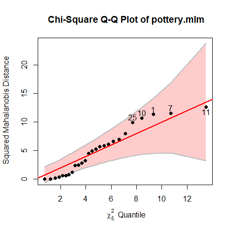

Figure 3: Chisquare QQ plot for the Pottery model.

Influence plot: An influence plot for this model, done using mvinfluence::influencePlot() plots the leverage multivariate hat-values for the predictors (site) against squared multivariate studentized residuals, using the size of the point symbol proportional to a multivariate generalization of Cook’s D statistic.

res <- influencePlot(pottery.mlm, id.n = 2)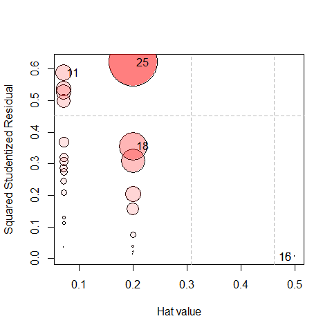

Figure 4: Influence plot for the Pottery model.

res |>
  arrange(desc(CookD))
#>          H        Q   CookD       L       R
#> 25 0.20000 0.621766 0.68394 0.25000 0.77721
#> 18 0.20000 0.355067 0.39057 0.25000 0.44383
#> 11 0.07143 0.587152 0.23067 0.07692 0.63232
#> 16 0.50000 0.006379 0.01754 1.00000 0.01276
#> 15 0.50000 0.006379 0.01754 1.00000 0.01276

Because site is a factor, the hat-values are inversely proportional to the sample size. Points for Llanedryn ( $n=14$ ) are in the left-most column, followed by AshleyRails and IsleThorns (each with $n=5$ ) and then Caldicot ( $n=14$ ).

Here, case 25 stands out with the largest value of Cook’s D, followed by 18 and 11.

Robust MANOVA

Now, fit the robust model using robmlm(). Because this uses an interative IRLS method, points that might not seem unusual in the initial model can become more noteworthy when the extreme observations are down-weighted in a subsequent iteration.

# Robust MANOVA model
pottery.rlm <- robmlm(cbind(Al, Fe, Mg, Ca, Na) ~ Site, data = Pottery)
Anova(pottery.rlm)
#> 
#> Type II MANOVA Tests: Pillai test statistic
#>      Df test stat approx F num Df den Df  Pr(>F)    
#> Site  3      1.98     6.55     15     51 1.7e-07 ***
#> ---
#> Signif. codes:  0 '***' 0.001 '**' 0.01 '*' 0.05 '.' 0.1 ' ' 1

Let’s compare the results. From the results of Anova() above, you can see that the $F$ statistic for the robust model is greater than that for OLS, which suggests that possible outliers may have reduced the strength of evidence for differences among the sites.

It is useful to compare the coefficients of the two models, and for this, their relative difference is a useful metric. The simple function reldiff() expresses these as the signed percent of difference between the classical and robust estimatges

b.mlm <- coef(pottery.mlm)
b.rlm <- coef(pottery.rlm)

reldiff <- function(x, y, pct=TRUE) {
  res <- abs(x - y) / x
  if (pct) res <- 100 * res
  res
}

reldiff(b.mlm, b.rlm)
#>                     Al      Fe      Mg      Ca      Na
#> (Intercept)      3.616  20.480  2.5908  10.333  0.6925
#> SiteCaldicot   -11.145   7.934  0.4832   2.211 16.6192
#> SiteIsleThorns  64.510 136.881 25.1469 -21.792  1.9605
#> SiteLlanedyrn  -11.559   9.969  2.0078   6.241 22.7443

Among these, the coefficients for IsleThorns are quite different for most of the variables.

Examining the Robust Weights

The robust fitting procedure assigns weights to each observation based on their deviation from the fitted model. Observations that appear to be outliers receive lower weights. The plot() method for a "roblm" object gives an index plot of the weight values.

# Plot the weights from robust fitting
plot(pottery.rlm, col=Pottery$Site, segments=TRUE)
xloc <- c(7.5, 15.5, 19.5, 24)
text(xloc, rep(c(1.0, 1.05), length=5), 
     levels(Pottery$Site), pos =3, xpd = TRUE)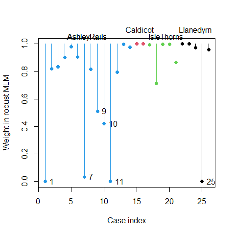

Figure 5: Weights from robust MANOVA fitting showing potential outliers

The weight plot reveals which observations were considered potentially problematic during the robust fitting process. Observations with weights substantially below 1.0 were down-weighted, indicating they may be outliers in the multivariate space defined by the five chemical measurements.

Hypothesis-Error (HE) plots

HE plots provide a visual representation of the multivariate hypothesis test by showing the relationship between hypothesis and error variation in a reduced dimensional space. We’ll create HE plots for the first two variables (Al and Fe) and compare the classical and robust fits.

# Classical HE plot for Al and Fe
heplot(pottery.mlm, variables = c("Al", "Fe"), 
       main = "Classical vs Robust MANOVA: Al vs Fe",
       col = c("blue", "blue"), fill = TRUE, fill.alpha = 0.2)

# Overlay robust HE plot
heplot(pottery.rlm, variables = c("Al", "Fe"), 
       add = TRUE, error.ellipse = TRUE,
       col = c("red", "red"), 
       fill = TRUE, fill.alpha = 0.2, lty = 2)

# Add legend
legend("topright", 
       legend = c("Classical", "Robust"), 
       col = c("blue", "red"), 
       lty = c(1, 2), 
       fill = c("blue", "red")
       )

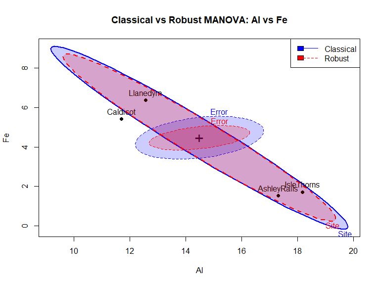
Figure 6: HE plot comparing classical (blue) and robust (red) MANOVA for Al vs Fe

The H and E ellipses have approximately the same shape and orientation for the classical and robust models, indicating that the pattern of differences among the group means is quite similar for both models. However, the E ellipse for the robust model is noticeably smaller. This goes into the greater $F$ statistic for the robust model.

For a more complete interpretation of robust model, a scatterplot matrix of HE plots is shown below, using the pairs() method for a MLM.

pairs(pottery.rlm, 
      fill=TRUE, fill.alpha = 0.1)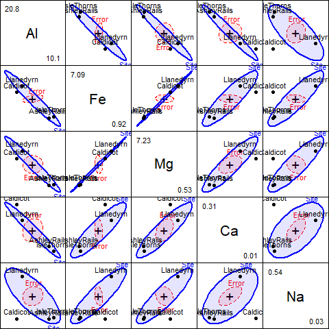

Figure 7: Pairwise HE plots for all response variables in the robust model pottery.rlm

Interpretation and Discussion

Several important insights emerge from this analysis of the Pottery data

Model evaluation: The comparison of MANOVA results shows …

Outlier detection: The weight plot identifies specific observations that deviate from the typical pattern. In archaeological studies, such outliers might represent pottery from different time periods, contaminated samples, or measurement errors that warrant further investigation.
Geometric interpretation: The HE plot comparison reveals how outliers affect the geometric representation of the hypothesis test. The hypothesis ellipse (representing the Site effect) and error ellipse (representing within-group variation) may differ substantially between classical and robust fits when influential outliers are present.
Practical implications: For archaeologists studying pottery composition, the robust analysis provides more reliable conclusions about site differences by reducing the influence of potentially problematic observations. This is particularly important when making inferences about ancient trade routes, cultural practices, or chronological relationships based on chemical composition data.

The robust approach demonstrates its value by providing a more stable analysis that is less susceptible to the influence of outlying observations, while still maintaining high efficiency when the data conform to standard assumptions.

References

Huber, P. J. (1964). Robust estimation of a location parameter. The Annals of Mathematical Statistics, 35(1), 73–101.

Rousseeuw, P. J., Van Aelst, S., Van Driessen, K., & Gulló, J. A. (2004). Robust multivariate regression. Technometrics, 46(3), 293–305. http://doi.org/10.1198/004017004000000329

Rousseeuw, P. J., & Yohai, V. J. (1984). Robust regression by means of S-estimators. In J. Franke, W. Härdle, & D. Martin (Eds.), Robust and nonlinear time series analysis (Vol. 26, pp. 256–272). New York: Springer.

Tukey, J. W. (1960). A survey of sampling from contaminated distributions.

Yohai, V. J. (1987). High breakdown-point and high efficiency robust estimates for regression. The Annals of Statistics, 15(2), 642–656.

Michael Friendly

2025-08-07