Taste Ratings of Japanese Rice Wine (Sake)

Siotani et al. (1985) describe a study of Japanese rice wine (sake) used to investigate the relationship between two subjective ratings (taste and smell) and a number of physical measurements on 30 brands of sake.

Format

A data frame with 30 observations on the following 10 variables.

taste: mean taste rating
smell: mean smell rating
pH: pH measurement
acidity1: one measure of acidity
acidity2: another measure of acidity
sake: Sake-meter score
rsugar: direct reducing sugar content
tsugar: total sugar content
alcohol: alcohol content
nitrogen: formol-nitrogen content

Source

Siotani, M. Hayakawa, T. & Fujikoshi, Y. (1985). Modern Multivariate Statistical Analysis: A Graduate Course and Handbook. American Sciences Press, p. 217.

Details

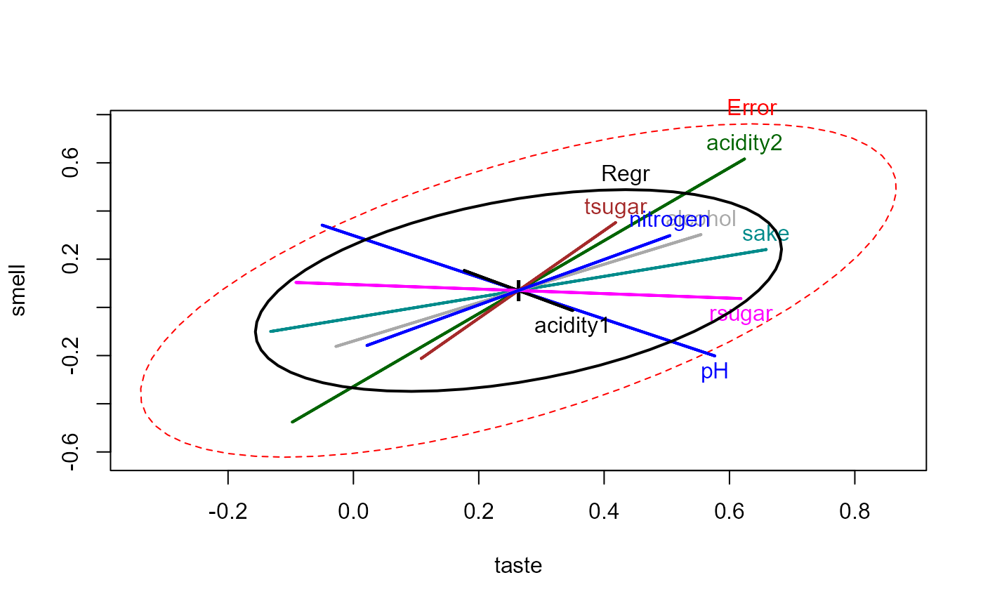
These data provide one example of a case where a multivariate regression doesn't benefit from having multiple outcome measures, using the standard tests. Barrett (2003) uses this data to illustrate influence measures for multivariate regression models.

The taste and smell values are the mean ratings of 10 experts on some unknown scale.

References

Barrett, B. E. (2003). Understanding Influence in Multivariate Regression. Communications in Statistics - Theory and Methods 32 (3), 667-680.

Examples


data(Sake)
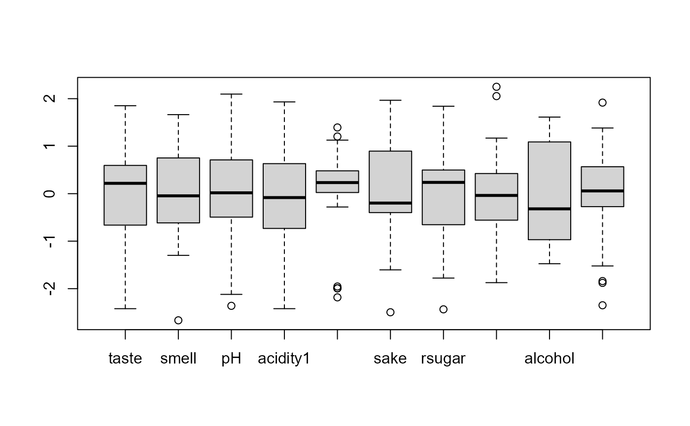
# quick look at the data
boxplot(scale(Sake))


Sake.mod <- lm(cbind(taste,smell) ~ ., data=Sake)

library(car)
car::Anova(Sake.mod)
#> 
#> Type II MANOVA Tests: Pillai test statistic
#>          Df test stat approx F num Df den Df  Pr(>F)  
#> pH        1  0.276246   3.8169      2     20 0.03944 *
#> acidity1  1  0.030788   0.3177      2     20 0.73145  
#> acidity2  1  0.183297   2.2444      2     20 0.13202  
#> sake      1  0.141187   1.6440      2     20 0.21827  
#> rsugar    1  0.178200   2.1684      2     20 0.14050  
#> tsugar    1  0.054842   0.5802      2     20 0.56891  
#> alcohol   1  0.075954   0.8220      2     20 0.45387  
#> nitrogen  1  0.056486   0.5987      2     20 0.55909  
#> ---
#> Signif. codes:  0 '***' 0.001 '**' 0.01 '*' 0.05 '.' 0.1 ' ' 1

predictors <- colnames(Sake)[-(1:2)]                 
# overall multivariate regression test
linearHypothesis(Sake.mod, predictors)
#> 
#> Sum of squares and products for the hypothesis:
#>           taste     smell
#> taste 1.4171079 0.5786338
#> smell 0.5786338 1.4095094
#> 
#> Sum of squares and products for error:
#>          taste    smell
#> taste 3.172559 2.248366
#> smell 2.248366 4.173491
#> 
#> Multivariate Tests: 
#>                  Df test stat approx F num Df den Df  Pr(>F)
#> Pillai            8 0.6300580 1.207279     16     42 0.30236
#> Wilks             8 0.4642360 1.169193     16     40 0.33210
#> Hotelling-Lawley  8 0.9509599 1.129265     16     38 0.36489
#> Roy               8 0.6270207 1.645929      8     21 0.17134

heplot(Sake.mod, hypotheses=list("Regr" = predictors))