The hospital manpower data, taken from Myers (1990), table 3.8, are a well-known example of highly collinear data to which ridge regression and various shrinkage and selection methods are often applied.
The data consist of measures taken at 17 U.S. Naval Hospitals and the goal is to predict the required monthly man hours for staffing purposes.
Format
A data frame with 17 observations on the following 6 variables.
Hoursmonthly man hours (response variable)
Loadaverage daily patient load
Xraymonthly X-ray exposures
BedDaysmonthly occupied bed days
AreaPopeligible population in the area in thousands
Stayaverage length of patient's stay in days
Source
Raymond H. Myers (1990). Classical and Modern Regression with Applications, 2nd ed., PWS-Kent, pp. 130-133.
Details
Myers (1990) indicates his source was "Procedures and Analysis for Staffing Standards Development: Data/Regression Analysis Handbook", Navy Manpower and Material Analysis Center, San Diego, 1979.
References
Donald R. Jensen and Donald E. Ramirez (2012). Variations on Ridge Traces in Regression, Communications in Statistics - Simulation and Computation, 41 (2), 265-278.
See also
manpower for the same data, and other
analyses
Examples
data(Manpower)
mmod <- lm(Hours ~ ., data=Manpower)
vif(mmod)
#> Load Xray BedDays AreaPop Stay
#> 9597.570761 7.940593 8933.086501 23.293856 4.279835
# ridge regression models, specified in terms of equivalent df
mridge <- ridge(Hours ~ ., data=Manpower, df=seq(5, 3.75, -.25))
vif(mridge)
#> Variance inflaction factors:
#> Load Xray BedDays AreaPop Stay
#> 0.0000000000 9597.571 7.941 8933.087 23.294 4.280
#> 0.0002836352 5602.507 7.927 5215.176 19.045 3.923
#> 0.0009043689 2438.604 7.913 2270.762 15.668 3.638
#> 0.0026667276 634.529 7.891 591.832 13.699 3.468
#> 0.0203643899 23.624 7.715 23.250 12.531 3.313
#> 0.1364900421 7.337 6.733 8.136 9.838 2.796
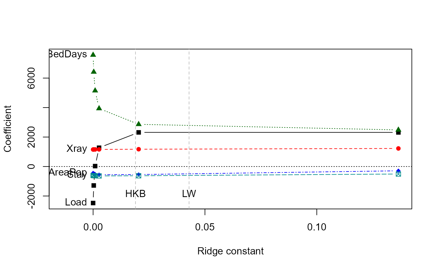
# univariate ridge trace plots
traceplot(mridge)
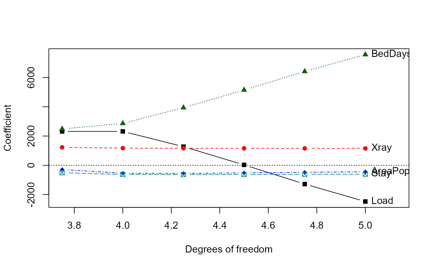
 traceplot(mridge, X="df")
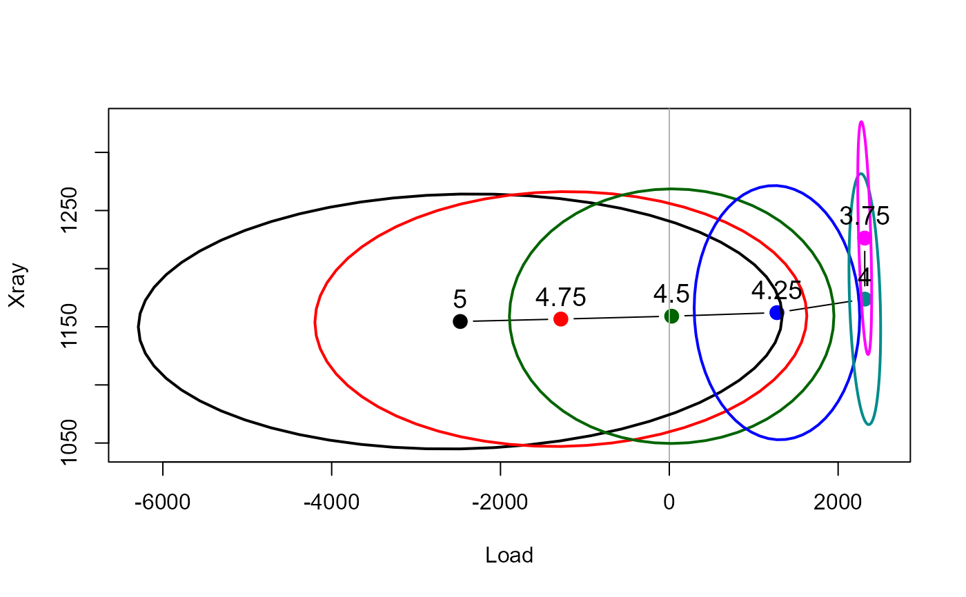
 # bivariate ridge trace plots
plot(mridge, radius=0.25, labels=mridge$df)
# bivariate ridge trace plots
plot(mridge, radius=0.25, labels=mridge$df)
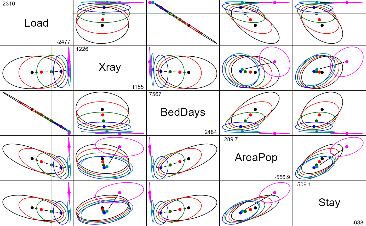
 pairs(mridge, radius=0.25)
 # \donttest{
# 3D views
# ellipsoids for Load, Xray & BedDays are nearly 2D
plot3d(mridge, radius=0.2, labels=mridge$df)
# variables in model selected by AIC & BIC
plot3d(mridge, variables=c(2,3,5), radius=0.2, labels=mridge$df)
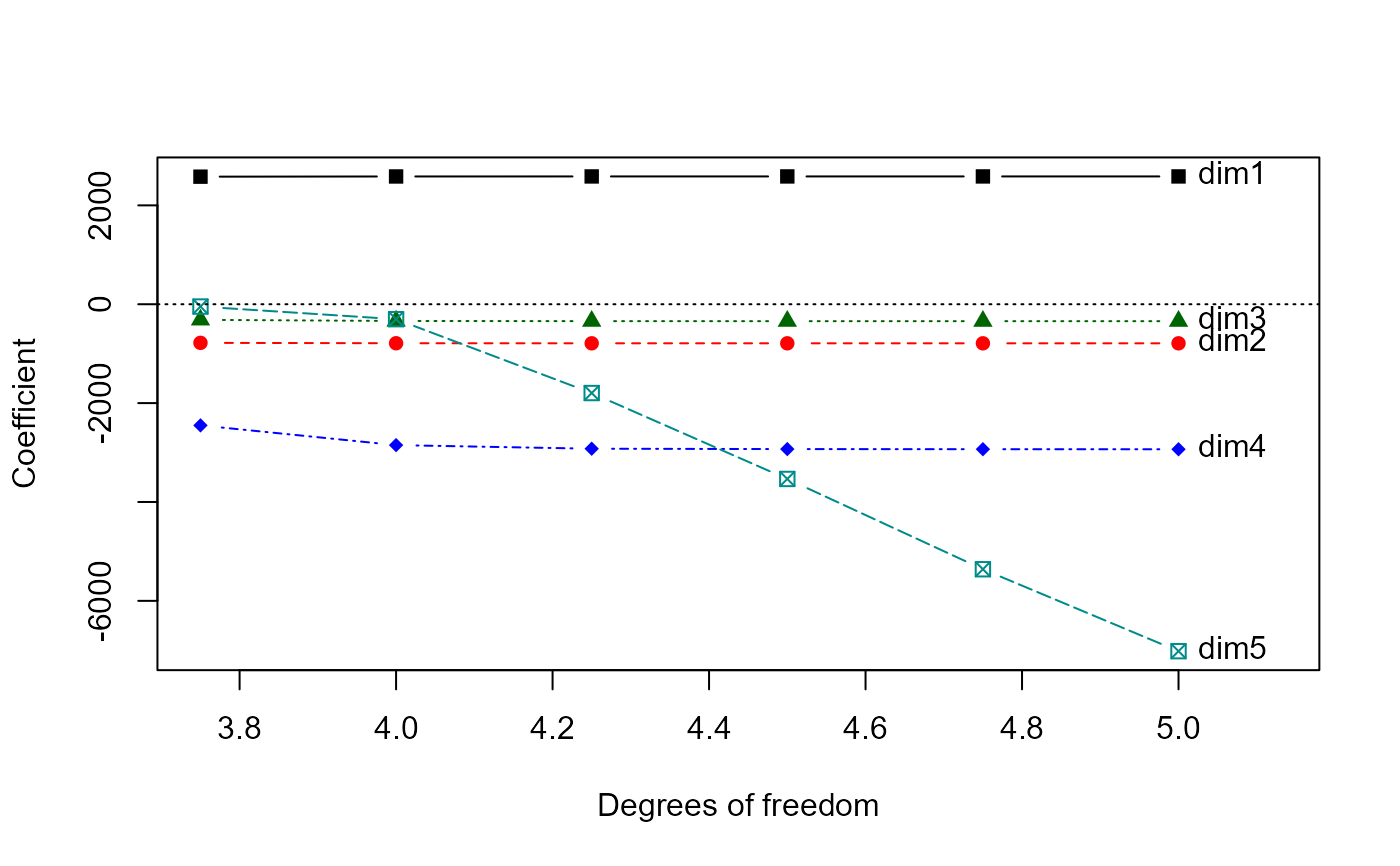
# plots in PCA/SVD space
mpridge <- pca(mridge)
traceplot(mpridge, X="df")
# \donttest{
# 3D views
# ellipsoids for Load, Xray & BedDays are nearly 2D
plot3d(mridge, radius=0.2, labels=mridge$df)
# variables in model selected by AIC & BIC
plot3d(mridge, variables=c(2,3,5), radius=0.2, labels=mridge$df)
# plots in PCA/SVD space
mpridge <- pca(mridge)
traceplot(mpridge, X="df")
 biplot(mpridge, radius=0.25)
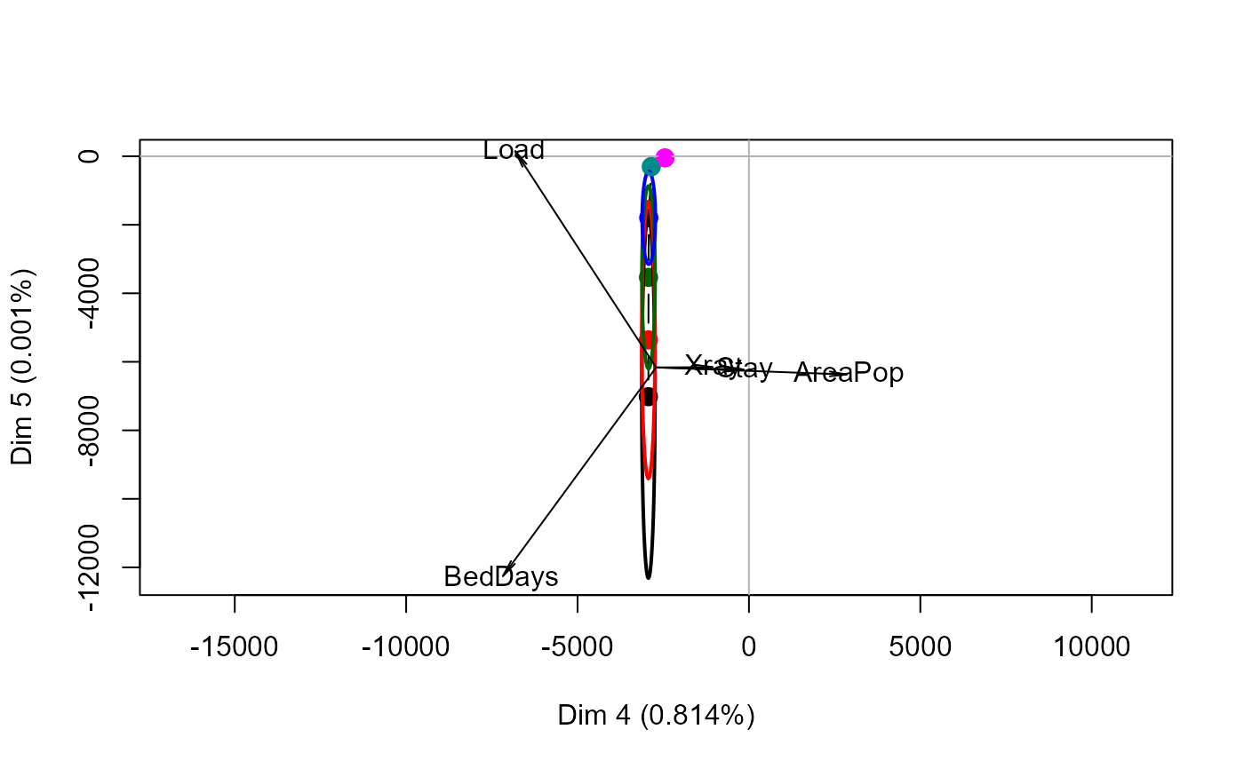 #> Vector scale factor set to 8774.365
# }
#> Vector scale factor set to 8774.365
# }