Univariate Ridge Trace Plots

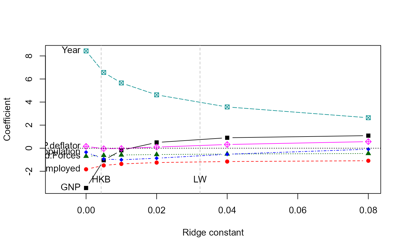
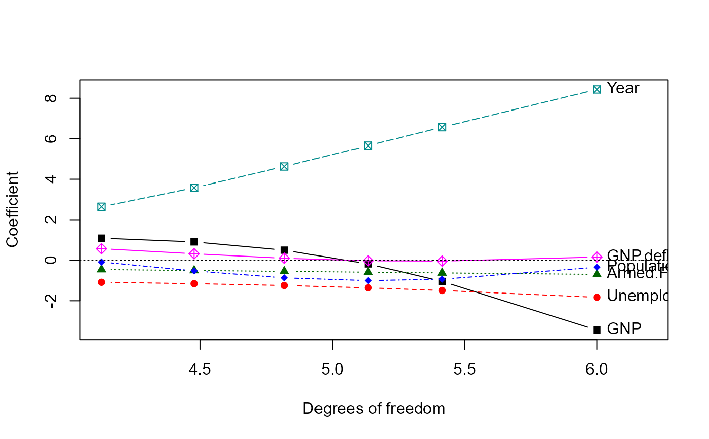
The traceplot function extends and simplifies the univariate ridge trace plots for ridge regression provided in the plot method for lm.ridge

Usage

traceplot(
  x,
  X = c("lambda", "df"),
  col = c("black", "red", "darkgreen", "blue", "darkcyan", "magenta", "brown",
    "darkgray"),
  pch = c(15:18, 7, 9, 12, 13),
  xlab,
  ylab = "Coefficient",
  xlim,
  ylim,
  ...
)

Arguments

x: A ridge object, as fit by ridge
X: What to plot as the horizontal coordinate, one of c("lambda", "df")
col: A numeric or character vector giving the colors used to plot the ridge trace curves. Recycled as necessary.
pch: Vector of plotting characters used to plot the ridge trace curves. Recycled as necessary.
xlab: Label for horizontal axis
ylab: Label for vertical axis
xlim, ylim: x, y limits for the plot. You may need to adjust these to allow for the variable labels.
...: Other arguments passed to matplot

Value

None. Used for its side effect of plotting.

Details

For ease of interpretation, the variables are labeled at the side of the plot (left, right) where the coefficient estimates are expected to be most widely spread. If xlim is not specified, the range of the X variable is extended slightly to accommodate the variable names.

References

Friendly, M. (2013). The Generalized Ridge Trace Plot: Visualizing Bias and Precision. Journal of Computational and Graphical Statistics, 22(1), 50-68, doi:10.1080/10618600.2012.681237, https://www.datavis.ca/papers/genridge-jcgs.pdf

Hoerl, A. E. and Kennard R. W. (1970). "Ridge Regression: Applications to Nonorthogonal Problems", Technometrics, 12(1), 69-82.

Author

Michael Friendly

Examples


longley.y <- longley[, "Employed"]
longley.X <- data.matrix(longley[, c(2:6,1)])

lambda <- c(0, 0.005, 0.01, 0.02, 0.04, 0.08)
lridge <- ridge(longley.y, longley.X, lambda=lambda)

traceplot(lridge)

#abline(v=lridge$kLW, lty=3)
#abline(v=lridge$kHKB, lty=3)
#text(lridge$kLW, -3, "LW")
#text(lridge$kHKB, -3, "HKB")

traceplot(lridge, X="df")