Bivariate Ridge Trace Plots

The bivariate ridge trace plot displays 2D projections of the covariance ellipsoids for a set of ridge regression estimates indexed by a ridge tuning constant.

The centers of these ellipses show the bias induced for each parameter, and also how the change in the ridge estimate for one parameter is related to changes for other parameters.

The size and shapes of the covariance ellipses show directly the effect on precision of the estimates as a function of the ridge tuning constant.

plot.pcaridge does these bivariate ridge trace plots for "pcaridge" objects, defaulting to plotting the two smallest components.

Usage

# S3 method for class 'ridge'
plot(
  x,
  variables = 1:2,
  radius = 1,
  which.lambda = 1:length(x$lambda),
  labels = lambda,
  pos = 3,
  cex = 1.2,
  lwd = 2,
  lty = 1,
  xlim,
  ylim,
  col = c("black", "red", "darkgreen", "blue", "darkcyan", "magenta", "brown",
    "darkgray"),
  center.pch = 16,
  center.cex = 1.5,
  fill = FALSE,
  fill.alpha = 0.3,
  ref = TRUE,
  ref.col = gray(0.7),
  ...
)

# S3 method for class 'pcaridge'
plot(x, variables = (p - 1):p, labels = NULL, ...)

Arguments

x: A ridge object, as fit by ridge
variables: Predictors in the model to be displayed in the plot: an integer or character vector of length 2, giving the indices or names of the variables. Defaults to the first two predictors for ridge objects or the last two dimensions for pcaridge objects.
radius: Radius of the ellipse-generating circle for the covariance ellipsoids. The default, radius=1 gives a standard “unit” ellipsoid. Typically, values radius<1 gives less cluttered displays.
which.lambda: A vector of indices used to select the values of lambda for which ellipses are plotted. The default is to plot ellipses for all values of lambda in the ridge object.
labels: A vector of character strings or expressions used as labels for the ellipses. Use labels=NULL to suppress these.
pos, cex: Scalars or vectors of positions (relative to the ellipse centers) and character size used to label the ellipses
lwd, lty: Line width and line type for the covariance ellipsoids. Recycled as necessary.
xlim, ylim: X, Y limits for the plot, each a vector of length 2. If missing, the range of the covariance ellipsoids is used.
col: A numeric or character vector giving the colors used to plot the covariance ellipsoids. Recycled as necessary.
center.pch: Plotting character used to show the bivariate ridge estimates. Recycled as necessary.
center.cex: Size of the plotting character for the bivariate ridge estimates
fill: Logical vector: Should the covariance ellipsoids be filled? Recycled as necessary.
fill.alpha: Numeric vector: alpha transparency value(s) in the range (0, 1) for filled ellipsoids. Recycled as necessary.
ref: Logical: whether to draw horizontal and vertical reference lines at 0.
ref.col: Color of reference lines.
...: Other arguments passed down to plot.default, e.g., xlab, ylab, and other graphic parameters.

Value

None. Used for its side effect of plotting.

References

Friendly, M. (2013). The Generalized Ridge Trace Plot: Visualizing Bias and Precision. Journal of Computational and Graphical Statistics, 22(1), 50-68, doi:10.1080/10618600.2012.681237, https://www.datavis.ca/papers/genridge-jcgs.pdf

Author

Michael Friendly

Examples


longley.y <- longley[, "Employed"]
longley.X <- data.matrix(longley[, c(2:6,1)])

lambda <- c(0, 0.005, 0.01, 0.02, 0.04, 0.08)
lambdaf <- c("", ".005", ".01", ".02", ".04", ".08")
lridge <- ridge(longley.y, longley.X, lambda=lambda)

op <- par(mfrow=c(2,2), mar=c(4, 4, 1, 1)+ 0.1)
for (i in 2:5) {
  plot(lridge, variables=c(1,i), radius=0.5, cex.lab=1.5)
  text(lridge$coef[1,1], lridge$coef[1,i], expression(~widehat(beta)^OLS), 
       cex=1.5, pos=4, offset=.1)
  if (i==2) text(lridge$coef[-1,1:2], lambdaf[-1], pos=3, cex=1.25)
}

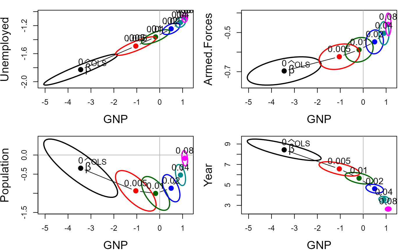par(op)

data(prostate)
py <- prostate[, "lpsa"]
pX <- data.matrix(prostate[, 1:8])
pridge <- ridge(py, pX, df=8:1)

plot(pridge)

plot(pridge, fill=c(TRUE, rep(FALSE,7)))