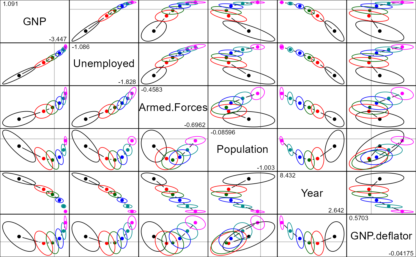
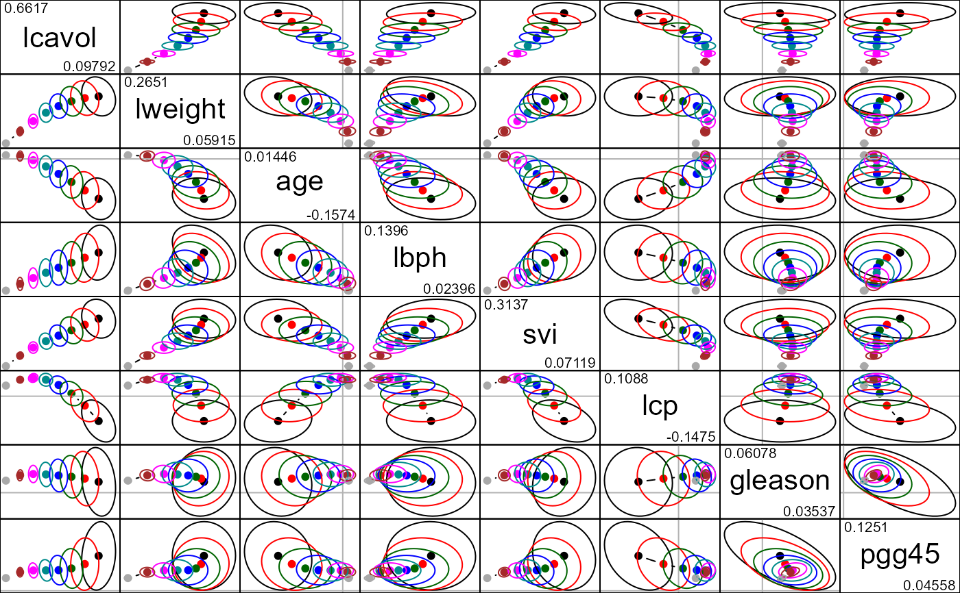
Displays all possible pairs of bivariate ridge trace plots for a given set of predictors.
Usage
# S3 method for class 'ridge'
pairs(
  x,
  variables,
  radius = 1,
  lwd = 1,
  lty = 1,
  col = c("black", "red", "darkgreen", "blue", "darkcyan", "magenta", "brown",
    "darkgray"),
  center.pch = 16,
  center.cex = 1.25,
  digits = getOption("digits") - 3,
  diag.cex = 2,
  diag.panel = panel.label,
  fill = FALSE,
  fill.alpha = 0.3,
  ...
)
Arguments
- x
A
ridgeobject, as fit byridge- variables
Predictors in the model to be displayed in the plot: an integer or character vector, giving the indices or names of the variables.
- radius
Radius of the ellipse-generating circle for the covariance ellipsoids.
- lwd, lty
Line width and line type for the covariance ellipsoids. Recycled as necessary.
- col
A numeric or character vector giving the colors used to plot the covariance ellipsoids. Recycled as necessary.
- center.pch
Plotting character used to show the bivariate ridge estimates. Recycled as necessary.
- center.cex
Size of the plotting character for the bivariate ridge estimates
- digits
Number of digits to be displayed as the (min, max) values in the diagonal panels
- diag.cex
Character size for predictor labels in diagonal panels
- diag.panel
Function to draw diagonal panels. Not yet implemented: just uses internal
panel.labelto write the variable name and ranges.- fill
Logical vector: Should the covariance ellipsoids be filled? Recycled as necessary.
- fill.alpha
Numeric vector: alpha transparency value(s) for filled ellipsoids. Recycled as necessary.
- ...
Other arguments passed down
References
Friendly, M. (2013). The Generalized Ridge Trace Plot: Visualizing Bias and Precision. Journal of Computational and Graphical Statistics, 22(1), 50-68, doi:10.1080/10618600.2012.681237, https://www.datavis.ca/papers/genridge-jcgs.pdf
See also
ridge for details on ridge regression as implemented here
plot.ridge, traceplot for other plotting methods
Examples
longley.y <- longley[, "Employed"]
longley.X <- data.matrix(longley[, c(2:6,1)])

lambda <- c(0, 0.005, 0.01, 0.02, 0.04, 0.08)
lridge <- ridge(longley.y, longley.X, lambda=lambda)

pairs(lridge, radius=0.5, diag.cex=1.75)


data(prostate)
py <- prostate[, "lpsa"]
pX <- data.matrix(prostate[, 1:8])
pridge <- ridge(py, pX, df=8:1)

pairs(pridge)

