The function ridge fits linear models by ridge regression, returning
an object of class ridge designed to be used with the plotting
methods in this package.
It is also designed to facilitate an alternative representation of the effects of shrinkage in the space of uncorrelated (PCA/SVD) components of the predictors.
The standard formulation of ridge regression is that it regularizes the estimates of coefficients by adding small positive constants \(\lambda\) to the diagonal elements of \(\mathbf{X}^\top\mathbf{X}\) in the least squares solution to achieve a more favorable tradeoff between bias and variance (inverse of precision) of the coefficients.
$$\widehat{\mathbf{\beta}}^{\text{RR}}_k = (\mathbf{X}^\top \mathbf{X} + \lambda \mathbf{I})^{-1} \mathbf{X}^\top \mathbf{y} $$
Ridge regression shrinkage can be parameterized in several ways.
If a vector of
lambdavalues is supplied, these are used directly in the ridge regression computations.Otherwise, if a vector
dfcan be supplied the equivalent values for effective degrees of freedom corresponding to shrinkage, going down from the number of predictors in the model.
In either case, both lambda and
df are returned in the ridge object, but the rownames of the
coefficients are given in terms of lambda.
coef extracts the estimated coefficients for each value of the shrinkage factor
vcov extracts the estimated \(p \times p\) covariance matrices of the coefficients for each value of the shrinkage factor.
best extracts the optimal shrinkage values according to several criteria:
HKB: Hoerl et al. (1975); LW: Lawless & Wang (1976); GCV: Golub et al. (1975)
Usage
ridge(y, ...)

# S3 method for class 'formula'
ridge(formula, data, lambda = 0, df, svd = TRUE, contrasts = NULL, ...)

# Default S3 method
ridge(y, X, lambda = 0, df, svd = TRUE, ...)

# S3 method for class 'ridge'
coef(object, ...)

# S3 method for class 'ridge'
print(x, digits = max(5, getOption("digits") - 5), ...)

# S3 method for class 'ridge'
vcov(object, ...)

best(object, ...)

# S3 method for class 'ridge'
best(object, ...)
Arguments
- y
A numeric vector containing the response variable. NAs not allowed.
- ...
Other arguments, passed down to methods
- formula
For the
formulamethod, a two-sided formula.- data
For the
formulamethod, data frame within which to evaluate the formula.- lambda
A scalar or vector of ridge constants. A value of 0 corresponds to ordinary least squares.
- df
A scalar or vector of effective degrees of freedom corresponding to
lambda- svd
If
TRUEthe SVD of the centered and scaledXmatrix is returned in theridgeobject.- contrasts
a list of contrasts to be used for some or all of factor terms in the formula. See the
contrasts.argofmodel.matrix.default.- X
A matrix of predictor variables. NA's not allowed. Should not include a column of 1's for the intercept.
- x, object
An object of class
ridge- digits
For the
printmethod, the number of digits to print.
Value
A list with the following components:
- lambda
The vector of ridge constants
- df
The vector of effective degrees of freedom corresponding to
lambda- coef
The matrix of estimated ridge regression coefficients
- scales
scalings used on the X matrix
- kHKB
HKB estimate of the ridge constant
- kLW
L-W estimate of the ridge constant
- GCV
vector of GCV values
- kGCV
value of
lambdawith the minimum GCV- criteria
Collects the criteria
kHKB,kLW, andkGCVin a named vector
If svd==TRUE (the default), the following are also included:
- svd.D
Singular values of the
svdof the scaled X matrix- svd.U
Left singular vectors of the
svdof the scaled X matrix. Rows correspond to observations and columns to dimensions.- svd.V
Right singular vectors of the
svdof the scaled X matrix. Rows correspond to variables and columns to dimensions.
Details
If an intercept is present in the model, its coefficient is not penalized. (If you want to penalize an intercept, put in your own constant term and remove the intercept.)
The predictors are centered, but not (yet) scaled in this implementation.
A number of the methods in the package assume that lambda is a vector of shrinkage constants
increasing from lambda[1] = 0, or equivalently, a vector of df decreasing from \(p\).
References
Hoerl, A. E., Kennard, R. W., and Baldwin, K. F. (1975), "Ridge Regression: Some Simulations," Communications in Statistics, 4, 105-123.
Lawless, J.F., and Wang, P. (1976), "A Simulation Study of Ridge and Other Regression Estimators," Communications in Statistics, 5, 307-323.
Golub G.H., Heath M., Wahba G. (1979) Generalized cross-validation as a method for choosing a good ridge parameter. Technometrics, 21:215–223. https://doi.org/10.2307/1268518
See also
lm.ridge for other implementations of ridge regression
traceplot, plot.ridge,
pairs.ridge, plot3d.ridge, for 1D, 2D, 3D plotting methods
pca.ridge, biplot.ridge,
biplot.pcaridge for views in PCA/SVD space
precision.ridge for measures of shrinkage and precision
Examples
#\donttest{
# Longley data, using number Employed as response
longley.y <- longley[, "Employed"]
longley.X <- data.matrix(longley[, c(2:6,1)])
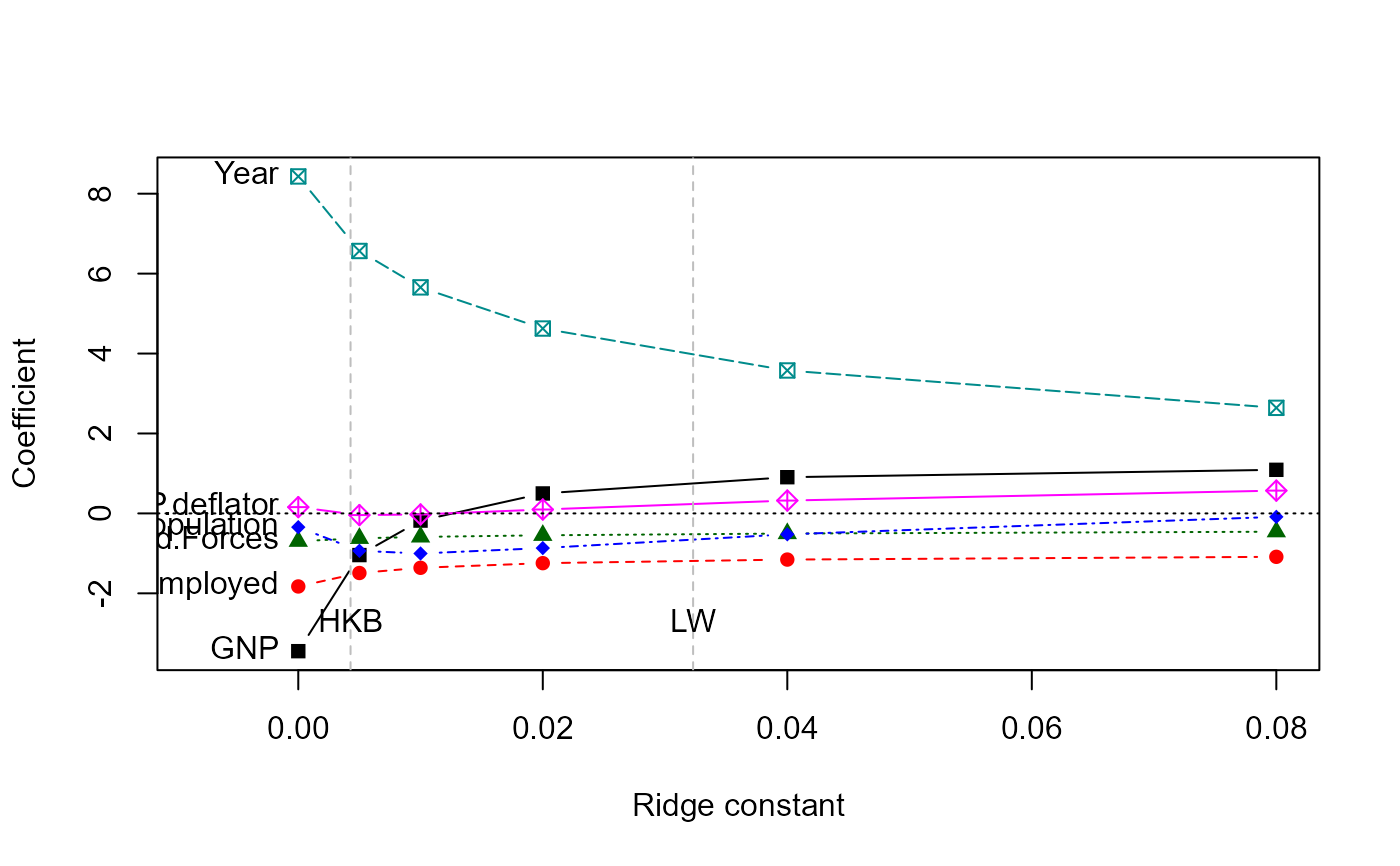
lambda <- c(0, 0.005, 0.01, 0.02, 0.04, 0.08)
lridge <- ridge(longley.y, longley.X, lambda=lambda)
# same, using formula interface
lridge <- ridge(Employed ~ GNP + Unemployed + Armed.Forces + Population + Year + GNP.deflator,
data=longley, lambda=lambda)
coef(lridge)
#> GNP Unemployed Armed.Forces Population Year GNP.deflator
#> 0.000 -3.4471925 -1.827886 -0.6962102 -0.34419721 8.431972 0.15737965
#> 0.005 -1.0424783 -1.491395 -0.6234680 -0.93558040 6.566532 -0.04175039
#> 0.010 -0.1797967 -1.361047 -0.5881396 -1.00316772 5.656287 -0.02612152
#> 0.020 0.4994945 -1.245137 -0.5476331 -0.86755299 4.626116 0.09766305
#> 0.040 0.9059471 -1.155229 -0.5039108 -0.52347060 3.576502 0.32123994
#> 0.080 1.0907048 -1.086421 -0.4582525 -0.08596324 2.641649 0.57025165
# standard trace plot
traceplot(lridge)
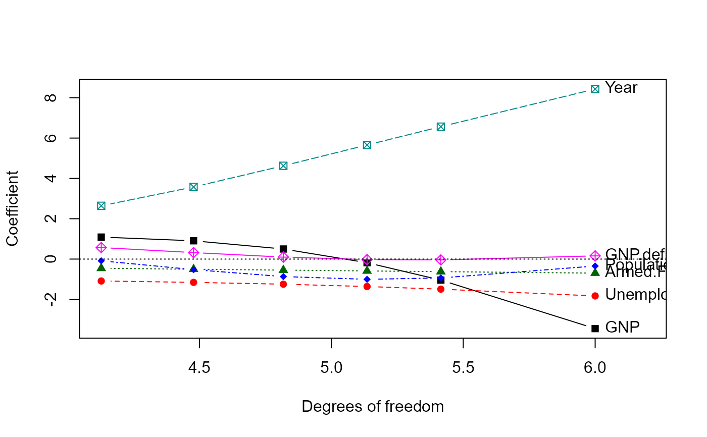
 # plot vs. equivalent df
traceplot(lridge, X="df")
# plot vs. equivalent df
traceplot(lridge, X="df")
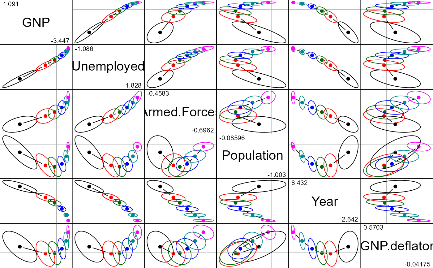
 pairs(lridge, radius=0.5)
 #}
# \donttest{
data(prostate)
py <- prostate[, "lpsa"]
pX <- data.matrix(prostate[, 1:8])
pridge <- ridge(py, pX, df=8:1)
pridge
#> Ridge Coefficients:
#> lcavol lweight age lbph svi
#> 0.00000 0.6617092 0.2651031 -0.1573777 0.1395860 0.3136993
#> 7.08544 0.5774912 0.2574888 -0.1240459 0.1239824 0.2825540
#> 17.80389 0.4966273 0.2435259 -0.0910692 0.1087544 0.2542261
#> 34.68940 0.4182786 0.2224269 -0.0591493 0.0936983 0.2271752
#> 62.98554 0.3413151 0.1935614 -0.0296600 0.0784146 0.1988651
#> 115.28893 0.2641305 0.1565931 -0.0049775 0.0622832 0.1660546
#> 230.11308 0.1842675 0.1116128 0.0112850 0.0444562 0.1249585
#> 601.44017 0.0979221 0.0591504 0.0144649 0.0239578 0.0711874
#> lcp gleason pgg45
#> 0.00000 -0.1475193 0.0353655 0.1250701
#> 7.08544 -0.0556184 0.0457910 0.0958079
#> 17.80389 0.0159166 0.0518160 0.0800300
#> 34.68940 0.0670223 0.0559538 0.0738953
#> 62.98554 0.0979877 0.0592922 0.0732073
#> 115.28893 0.1087550 0.0607835 0.0729838
#> 230.11308 0.0981548 0.0564920 0.0666687
#> 601.44017 0.0633002 0.0392473 0.0455834
plot(pridge)
#}
# \donttest{
data(prostate)
py <- prostate[, "lpsa"]
pX <- data.matrix(prostate[, 1:8])
pridge <- ridge(py, pX, df=8:1)
pridge
#> Ridge Coefficients:
#> lcavol lweight age lbph svi
#> 0.00000 0.6617092 0.2651031 -0.1573777 0.1395860 0.3136993
#> 7.08544 0.5774912 0.2574888 -0.1240459 0.1239824 0.2825540
#> 17.80389 0.4966273 0.2435259 -0.0910692 0.1087544 0.2542261
#> 34.68940 0.4182786 0.2224269 -0.0591493 0.0936983 0.2271752
#> 62.98554 0.3413151 0.1935614 -0.0296600 0.0784146 0.1988651
#> 115.28893 0.2641305 0.1565931 -0.0049775 0.0622832 0.1660546
#> 230.11308 0.1842675 0.1116128 0.0112850 0.0444562 0.1249585
#> 601.44017 0.0979221 0.0591504 0.0144649 0.0239578 0.0711874
#> lcp gleason pgg45
#> 0.00000 -0.1475193 0.0353655 0.1250701
#> 7.08544 -0.0556184 0.0457910 0.0958079
#> 17.80389 0.0159166 0.0518160 0.0800300
#> 34.68940 0.0670223 0.0559538 0.0738953
#> 62.98554 0.0979877 0.0592922 0.0732073
#> 115.28893 0.1087550 0.0607835 0.0729838
#> 230.11308 0.0981548 0.0564920 0.0666687
#> 601.44017 0.0633002 0.0392473 0.0455834
plot(pridge)
 pairs(pridge)
 traceplot(pridge)
 traceplot(pridge, X="df")
 # }
# Hospital manpower data from Table 3.8 of Myers (1990)
data(Manpower)
str(Manpower)
#> 'data.frame': 17 obs. of 6 variables:
#> $ Hours : num 567 697 1033 1604 1611 ...
#> $ Load : num 15.6 44 20.4 18.7 49.2 ...
#> $ Xray : int 2463 2048 3940 6505 5723 11520 5779 5969 8461 20106 ...
#> $ BedDays: num 473 1340 620 568 1498 ...
#> $ AreaPop: num 18 9.5 12.8 36.7 35.7 ...
#> $ Stay : num 4.45 6.92 4.28 3.9 5.5 4.6 5.62 5.15 6.18 6.15 ...
mmod <- lm(Hours ~ ., data=Manpower)
vif(mmod)
#> Load Xray BedDays AreaPop Stay
#> 9597.570761 7.940593 8933.086501 23.293856 4.279835
# ridge regression models, specified in terms of equivalent df
mridge <- ridge(Hours ~ ., data=Manpower, df=seq(5, 3.75, -.25))
vif(mridge)
#> Variance inflaction factors:
#> Load Xray BedDays AreaPop Stay
#> 0.0000000000 9597.571 7.941 8933.087 23.294 4.280
#> 0.0002836352 5602.507 7.927 5215.176 19.045 3.923
#> 0.0009043689 2438.604 7.913 2270.762 15.668 3.638
#> 0.0026667276 634.529 7.891 591.832 13.699 3.468
#> 0.0203643899 23.624 7.715 23.250 12.531 3.313
#> 0.1364900421 7.337 6.733 8.136 9.838 2.796
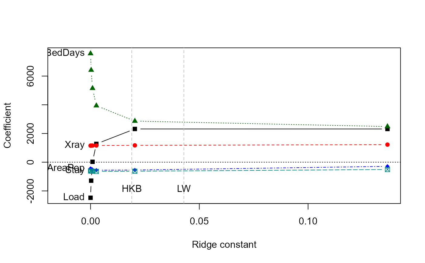
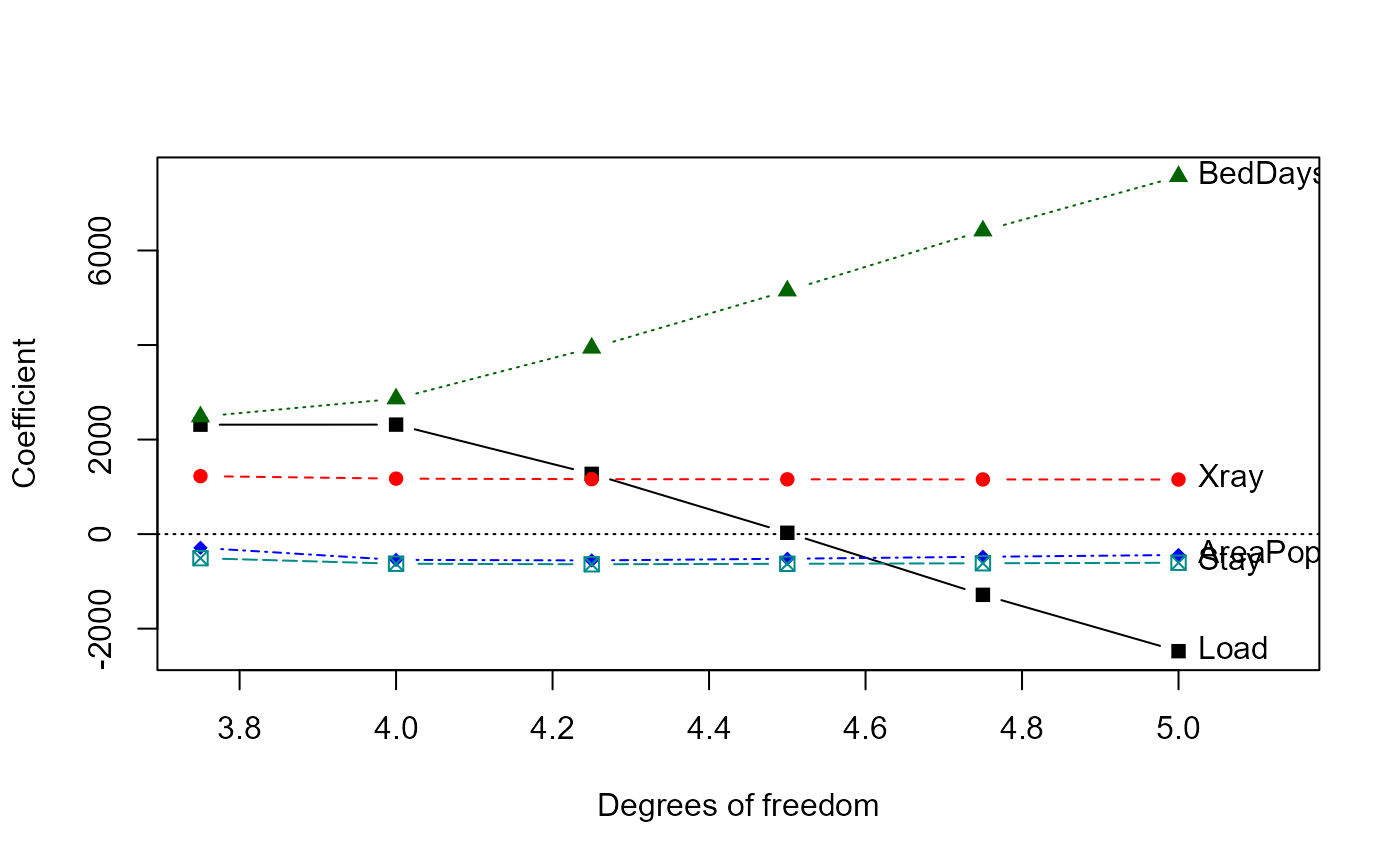
# univariate ridge trace plots
traceplot(mridge)
# }
# Hospital manpower data from Table 3.8 of Myers (1990)
data(Manpower)
str(Manpower)
#> 'data.frame': 17 obs. of 6 variables:
#> $ Hours : num 567 697 1033 1604 1611 ...
#> $ Load : num 15.6 44 20.4 18.7 49.2 ...
#> $ Xray : int 2463 2048 3940 6505 5723 11520 5779 5969 8461 20106 ...
#> $ BedDays: num 473 1340 620 568 1498 ...
#> $ AreaPop: num 18 9.5 12.8 36.7 35.7 ...
#> $ Stay : num 4.45 6.92 4.28 3.9 5.5 4.6 5.62 5.15 6.18 6.15 ...
mmod <- lm(Hours ~ ., data=Manpower)
vif(mmod)
#> Load Xray BedDays AreaPop Stay
#> 9597.570761 7.940593 8933.086501 23.293856 4.279835
# ridge regression models, specified in terms of equivalent df
mridge <- ridge(Hours ~ ., data=Manpower, df=seq(5, 3.75, -.25))
vif(mridge)
#> Variance inflaction factors:
#> Load Xray BedDays AreaPop Stay
#> 0.0000000000 9597.571 7.941 8933.087 23.294 4.280
#> 0.0002836352 5602.507 7.927 5215.176 19.045 3.923
#> 0.0009043689 2438.604 7.913 2270.762 15.668 3.638
#> 0.0026667276 634.529 7.891 591.832 13.699 3.468
#> 0.0203643899 23.624 7.715 23.250 12.531 3.313
#> 0.1364900421 7.337 6.733 8.136 9.838 2.796
# univariate ridge trace plots
traceplot(mridge)
 traceplot(mridge, X="df")
 # \donttest{
# bivariate ridge trace plots
plot(mridge, radius=0.25, labels=mridge$df)
# \donttest{
# bivariate ridge trace plots
plot(mridge, radius=0.25, labels=mridge$df)
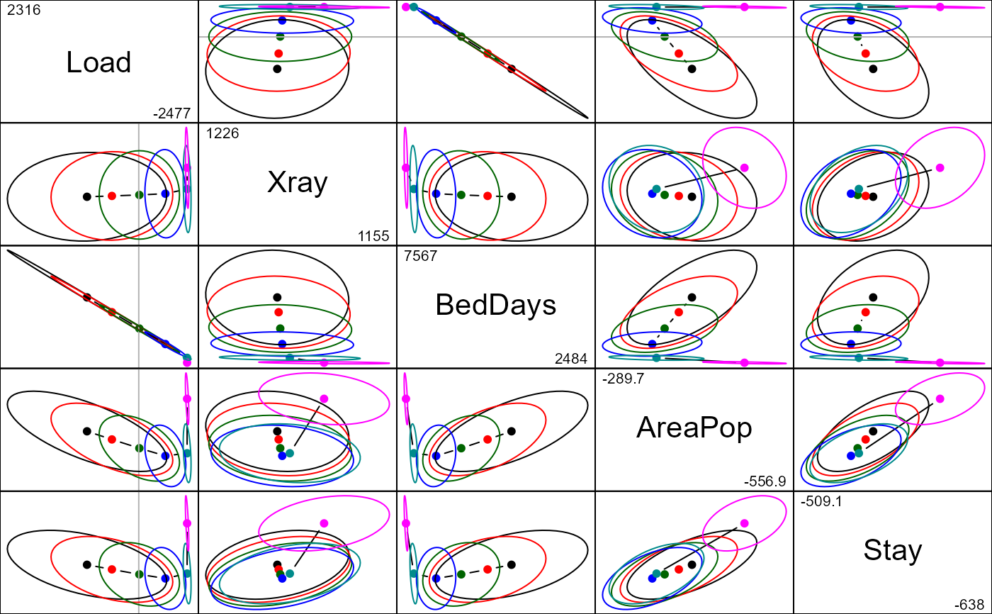
 pairs(mridge, radius=0.25)
 # 3D views
# ellipsoids for Load, Xray & BedDays are nearly 2D
plot3d(mridge, radius=0.2, labels=mridge$df)
# variables in model selected by AIC & BIC
plot3d(mridge, variables=c(2,3,5), radius=0.2, labels=mridge$df)
# plots in PCA/SVD space
mpridge <- pca(mridge)
traceplot(mpridge, X="df")
# 3D views
# ellipsoids for Load, Xray & BedDays are nearly 2D
plot3d(mridge, radius=0.2, labels=mridge$df)
# variables in model selected by AIC & BIC
plot3d(mridge, variables=c(2,3,5), radius=0.2, labels=mridge$df)
# plots in PCA/SVD space
mpridge <- pca(mridge)
traceplot(mpridge, X="df")
 biplot(mpridge, radius=0.25)
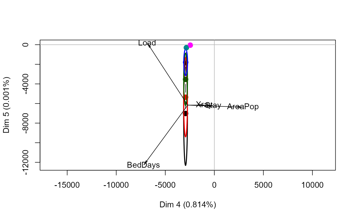 #> Vector scale factor set to 8774.365
# }
#> Vector scale factor set to 8774.365
# }