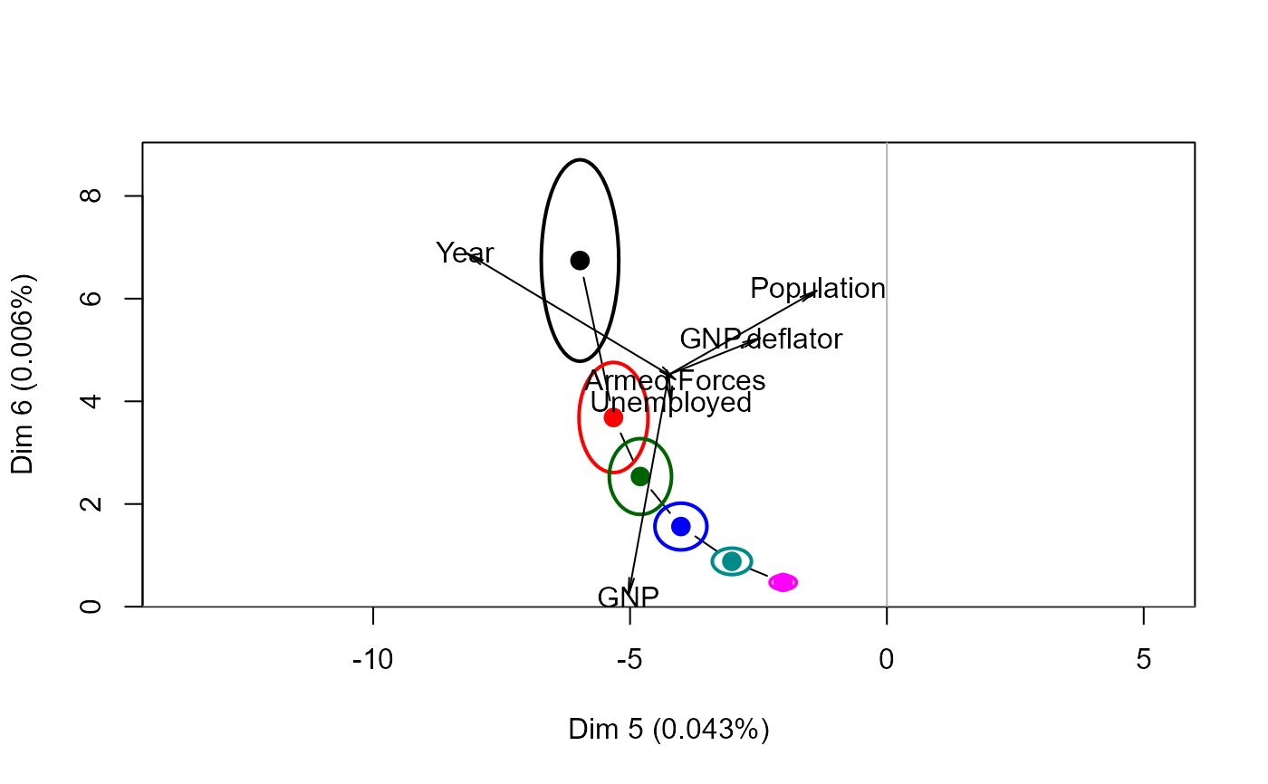
Biplot of Ridge Regression Trace Plot in SVD Space

biplot.pcaridge supplements the standard display of the covariance ellipsoids for a ridge regression problem in PCA/SVD space with labeled arrows showing the contributions of the original variables to the dimensions plotted.

Usage

# S3 method for class 'pcaridge'
biplot(
  x,
  variables = (p - 1):p,
  labels = NULL,
  asp = 1,
  origin,
  scale,
  var.lab = rownames(V),
  var.lwd = 1,
  var.col = "black",
  var.cex = 1,
  xlab,
  ylab,
  prefix = "Dim ",
  suffix = TRUE,
  ...
)

Arguments

x: A pcaridge object computed by pca.ridge or a ridge object.
variables: The dimensions or variables to be shown in the the plot. By default, the last two dimensions, corresponding to the smallest singular values, are plotted for class("pcaridge") objects or the first two variables for class("ridge") objects.
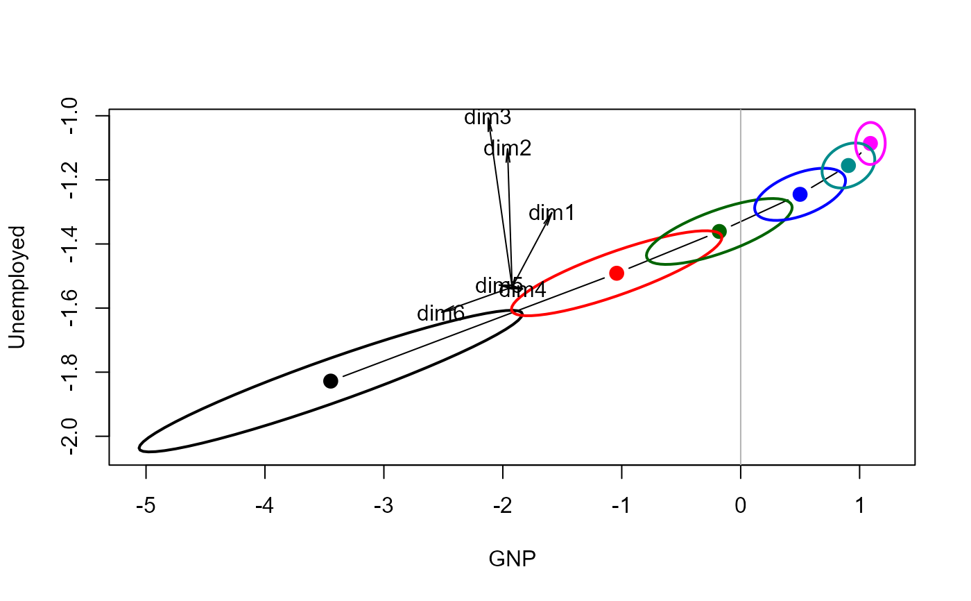
labels: A vector of character strings or expressions used as labels for the ellipses. Use labels=NULL to suppress these.
asp: Aspect ratio for the plot. The default value, asp=1 helps ensure that lengths and angles are preserved in these plots. Use asp=NA to override this.
origin: The origin for the variable vectors in this plot, a vector of length 2. If not specified, the function calculates an origin to make the variable vectors approximately centered in the plot window.
scale: The scale factor for variable vectors in this plot. If not specified, the function calculates a scale factor to make the variable vectors approximately fill the plot window.
var.lab: Labels for variable vectors. The default is the names of the predictor variables.
var.lwd, var.col, var.cex: Line width, color and character size used to draw and label the arrows representing the variables in this plot.
xlab, ylab: Labels for the plot dimensions. If not specified, prefix and suffix are used to construct informative dimension labels.
prefix: Prefix for labels of the plot dimensions.
suffix: Suffix for labels of the plot dimensions. If suffix=TRUE the percent of variance accounted for by each dimension is added to the axis label.
...: Other arguments, passed to plot.pcaridge

Value

None

Details

The biplot view showing the dimensions corresponding to the two smallest singular values is particularly useful for understanding how the predictors contribute to shrinkage in ridge regression.

This is only a biplot in the loose sense that results are shown in two spaces simultaneously – the transformed PCA/SVD space of the original predictors, and vectors representing the predictors projected into this space.

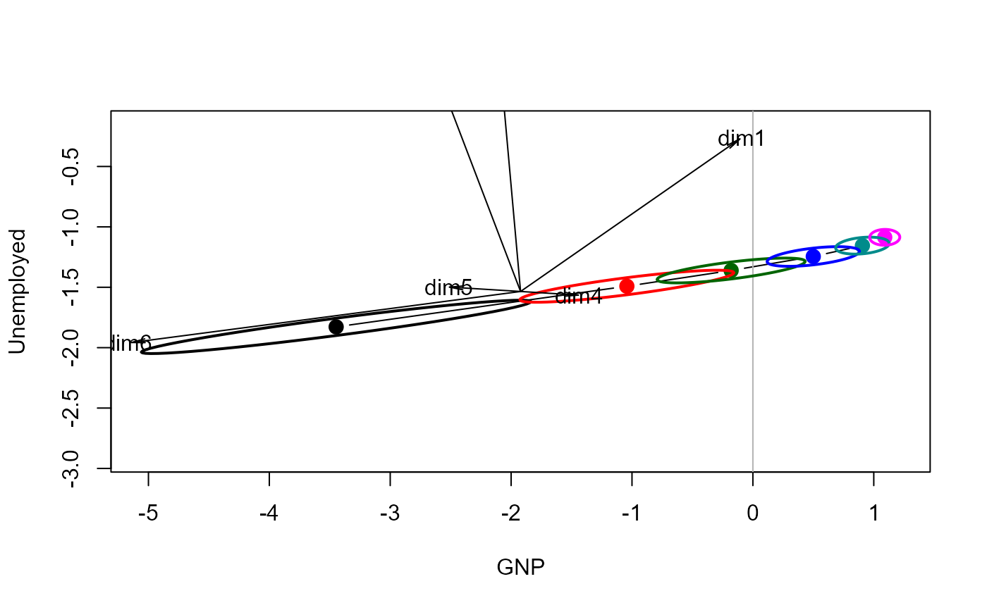
biplot.ridge is a similar extension of plot.ridge, adding vectors showing the relation of the PCA/SVD dimensions to the plotted variables.

class("ridge") objects use the transpose of the right singular vectors, t(x$svd.V) for the dimension weights plotted as vectors.

References

Friendly, M. (2013). The Generalized Ridge Trace Plot: Visualizing Bias and Precision. Journal of Computational and Graphical Statistics, 22(1), 50-68, doi:10.1080/10618600.2012.681237 , https://datavis.ca/papers/genridge-jcgs.pdf

Author

Michael Friendly, with contributions by Uwe Ligges

Examples


longley.y <- longley[, "Employed"]
longley.X <- data.matrix(longley[, c(2:6,1)])

lambda <- c(0, 0.005, 0.01, 0.02, 0.04, 0.08)
lridge <- ridge(longley.y, longley.X, lambda=lambda)

plridge <- pca(lridge)

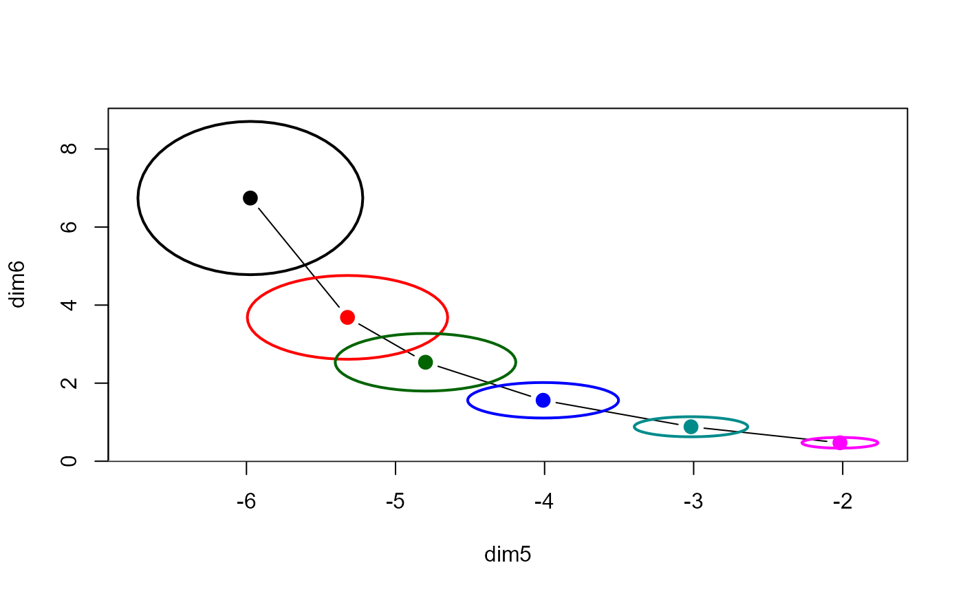
plot(plridge, radius=0.5)


# same, with variable vectors
biplot(plridge, radius=0.5)

#> Vector scale factor set to  5.246566 
# add some other options
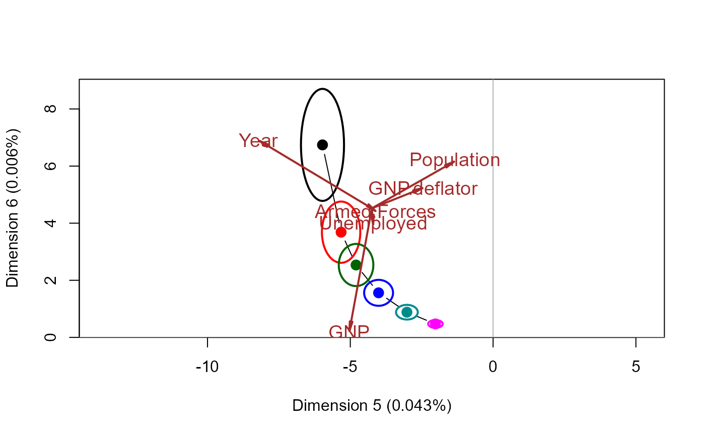
biplot(plridge, radius=0.5, var.col="brown", var.lwd=2, var.cex=1.2, prefix="Dimension ")

#> Vector scale factor set to  5.246566 

# biplots for ridge objects, showing PCA vectors
plot(lridge, radius=0.5)

biplot(lridge, radius=0.5)

#> Vector scale factor set to  3.932418 
biplot(lridge, radius=0.5, asp=NA)

#> Vector scale factor set to  0.7240638