Hauser (1979) presented this two-way frequency table, cross-classifying occupational categories of sons and fathers in the United States.
Format
A frequency data frame with 25 observations on the following 3 variables, representing the cross-classification of 19912 individuals by father's occupation and son's first occupation.
Sona factor with levels
UpNMLoNMUpMLoMFarmFathera factor with levels
UpNMLoNMUpMLoMFarmFreqa numeric vector
Source
R.M. Hauser (1979), Some exploratory methods for modeling mobility tables and other cross-classified data. In: K.F. Schuessler (Ed.), Sociological Methodology, 1980, Jossey-Bass, San Francisco, pp. 413-458. Table 1.
Details
It is a good example for exploring a variety of models for square tables: quasi-independence, quasi-symmetry, row/column effects, uniform association, etc., using the facilities of the gnm.
Hauser's data was first presented in 1979, and then published in 1980. The name of the dataset reflects the earliest use.
It reflects the "frequencies in a classification of son's first full-time civilian occupation by father's (or other family head's) occupation at son's sixteenth birthday among American men who were aged 20 to 64 in 1973 and were not currently enrolled in school".
As noted in Hauser's Table 1, "Counts are based on observations weighted to estimate population counts and compensate for departures of the sampling design from simple random sampling. Broad occupation groups are upper nonmanual: professional and kindred workers, managers and officials, and non-retail sales workers; lower nonmanual: proprietors, clerical and kindred workers, and retail sales workers; upper manual: craftsmen, foremen, and kindred workers; lower manual: service workers, operatives and kindred workers, and laborers (except farm); farm: farmers and farm managers, farm laborers, and foremen. density of mobility or immobility in the cells to which they refer."
The table levels for Son and Father have been arranged in
order of decreasing status as is common for mobility tables.
References
Powers, D.A. and Xie, Y. (2008). Statistical Methods for Categorical Data Analysis, Bingley, UK: Emerald.
Examples
data(Hauser79)
str(Hauser79)
#> 'data.frame': 25 obs. of 3 variables:
#> $ Son : Factor w/ 5 levels "UpNM","LoNM",..: 1 2 3 4 5 1 2 3 4 5 ...
#> $ Father: Factor w/ 5 levels "UpNM","LoNM",..: 1 1 1 1 1 2 2 2 2 2 ...
#> $ Freq : num 1414 521 302 643 40 ...
# display table
structable(~Father+Son, data=Hauser79)
#> Son UpNM LoNM UpM LoM Farm
#> Father
#> UpNM 1414 521 302 643 40
#> LoNM 724 524 254 703 48
#> UpM 798 648 856 1676 108
#> LoM 756 914 771 3325 237
#> Farm 409 357 441 1611 1832
#Examples from Powers & Xie, Table 4.15
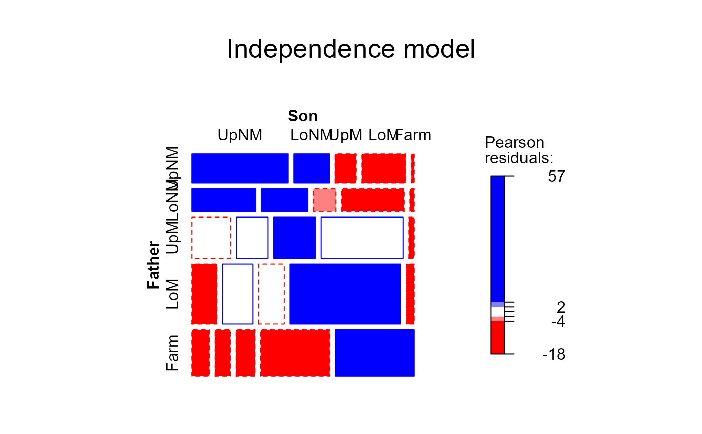
# independence model
mosaic(Freq ~ Father + Son, data=Hauser79, shade=TRUE)
 hauser.indep <- gnm(Freq ~ Father + Son,
data=Hauser79,
family=poisson)
mosaic(hauser.indep, ~Father+Son,
main="Independence model",
gp=shading_Friendly)
hauser.indep <- gnm(Freq ~ Father + Son,
data=Hauser79,
family=poisson)
mosaic(hauser.indep, ~Father+Son,
main="Independence model",
gp=shading_Friendly)
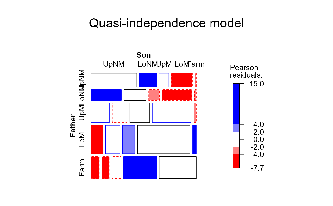
 # Quasi-independence
hauser.quasi <- update(hauser.indep,
~ . + Diag(Father,Son))
mosaic(hauser.quasi, ~Father+Son,
main="Quasi-independence model",
gp=shading_Friendly)
# Quasi-independence
hauser.quasi <- update(hauser.indep,
~ . + Diag(Father,Son))
mosaic(hauser.quasi, ~Father+Son,
main="Quasi-independence model",
gp=shading_Friendly)
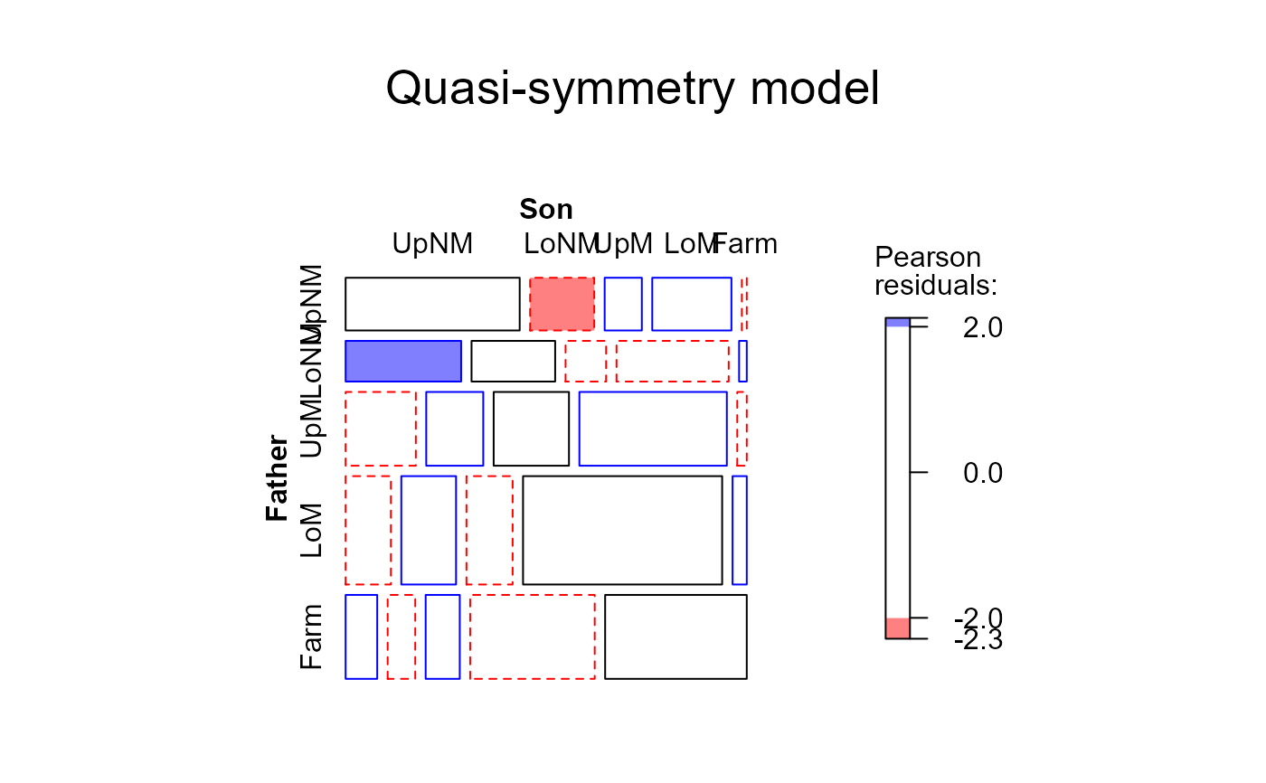
 # Quasi-symmetry
hauser.qsymm <- update(hauser.indep,
~ . + Diag(Father,Son) + Symm(Father,Son))
mosaic(hauser.qsymm, ~Father+Son,
main="Quasi-symmetry model",
gp=shading_Friendly)
# Quasi-symmetry
hauser.qsymm <- update(hauser.indep,
~ . + Diag(Father,Son) + Symm(Father,Son))
mosaic(hauser.qsymm, ~Father+Son,
main="Quasi-symmetry model",
gp=shading_Friendly)
 # numeric scores for row/column effects
Sscore <- as.numeric(Hauser79$Son)
Fscore <- as.numeric(Hauser79$Father)
# row effects model
hauser.roweff <- update(hauser.indep, ~ . + Father*Sscore)
LRstats(hauser.roweff)
#> Likelihood summary table:
#> AIC BIC LR Chisq Df Pr(>Chisq)
#> hauser.roweff 2308.9 2324.7 2080.2 12 < 2.2e-16 ***
#> ---
#> Signif. codes: 0 ‘***’ 0.001 ‘**’ 0.01 ‘*’ 0.05 ‘.’ 0.1 ‘ ’ 1
# uniform association
hauser.UA <- update(hauser.indep, ~ . + Fscore*Sscore)
LRstats(hauser.UA)
#> Likelihood summary table:
#> AIC BIC LR Chisq Df Pr(>Chisq)
#> hauser.UA 2503.4 2515.6 2280.7 15 < 2.2e-16 ***
#> ---
#> Signif. codes: 0 ‘***’ 0.001 ‘**’ 0.01 ‘*’ 0.05 ‘.’ 0.1 ‘ ’ 1
# uniform association, omitting diagonals
hauser.UAdiag <- update(hauser.indep, ~ . + Fscore*Sscore + Diag(Father,Son))
LRstats(hauser.UAdiag)
#> Likelihood summary table:
#> AIC BIC LR Chisq Df Pr(>Chisq)
#> hauser.UAdiag 305.72 324 73.007 10 1.161e-11 ***
#> ---
#> Signif. codes: 0 ‘***’ 0.001 ‘**’ 0.01 ‘*’ 0.05 ‘.’ 0.1 ‘ ’ 1
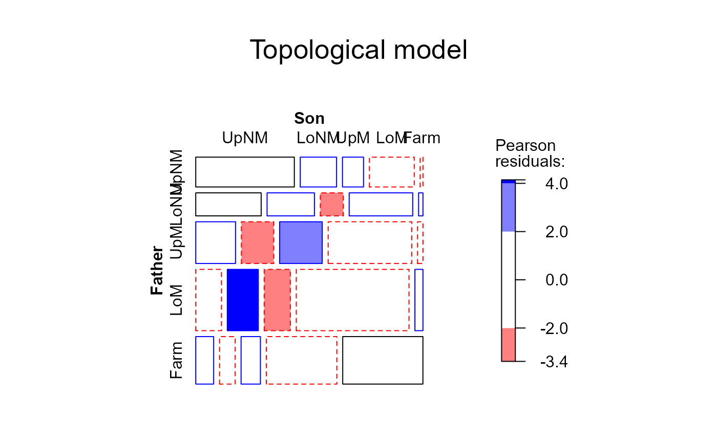
# Levels for Hauser 5-level model
levels <- matrix(c(
2, 4, 5, 5, 5,
3, 4, 5, 5, 5,
5, 5, 5, 5, 5,
5, 5, 5, 4, 4,
5, 5, 5, 4, 1
), 5, 5, byrow=TRUE)
hauser.topo <- update(hauser.indep,
~ . + Topo(Father, Son, spec=levels))
mosaic(hauser.topo, ~Father+Son,
main="Topological model", gp=shading_Friendly)
# numeric scores for row/column effects
Sscore <- as.numeric(Hauser79$Son)
Fscore <- as.numeric(Hauser79$Father)
# row effects model
hauser.roweff <- update(hauser.indep, ~ . + Father*Sscore)
LRstats(hauser.roweff)
#> Likelihood summary table:
#> AIC BIC LR Chisq Df Pr(>Chisq)
#> hauser.roweff 2308.9 2324.7 2080.2 12 < 2.2e-16 ***
#> ---
#> Signif. codes: 0 ‘***’ 0.001 ‘**’ 0.01 ‘*’ 0.05 ‘.’ 0.1 ‘ ’ 1
# uniform association
hauser.UA <- update(hauser.indep, ~ . + Fscore*Sscore)
LRstats(hauser.UA)
#> Likelihood summary table:
#> AIC BIC LR Chisq Df Pr(>Chisq)
#> hauser.UA 2503.4 2515.6 2280.7 15 < 2.2e-16 ***
#> ---
#> Signif. codes: 0 ‘***’ 0.001 ‘**’ 0.01 ‘*’ 0.05 ‘.’ 0.1 ‘ ’ 1
# uniform association, omitting diagonals
hauser.UAdiag <- update(hauser.indep, ~ . + Fscore*Sscore + Diag(Father,Son))
LRstats(hauser.UAdiag)
#> Likelihood summary table:
#> AIC BIC LR Chisq Df Pr(>Chisq)
#> hauser.UAdiag 305.72 324 73.007 10 1.161e-11 ***
#> ---
#> Signif. codes: 0 ‘***’ 0.001 ‘**’ 0.01 ‘*’ 0.05 ‘.’ 0.1 ‘ ’ 1
# Levels for Hauser 5-level model
levels <- matrix(c(
2, 4, 5, 5, 5,
3, 4, 5, 5, 5,
5, 5, 5, 5, 5,
5, 5, 5, 4, 4,
5, 5, 5, 4, 1
), 5, 5, byrow=TRUE)
hauser.topo <- update(hauser.indep,
~ . + Topo(Father, Son, spec=levels))
mosaic(hauser.topo, ~Father+Son,
main="Topological model", gp=shading_Friendly)
 # RC model
hauser.RC <- update(hauser.indep, ~ . + Mult(Father, Son), verbose=FALSE)
mosaic(hauser.RC, ~Father+Son, main="RC model", gp=shading_Friendly)
# RC model
hauser.RC <- update(hauser.indep, ~ . + Mult(Father, Son), verbose=FALSE)
mosaic(hauser.RC, ~Father+Son, main="RC model", gp=shading_Friendly)
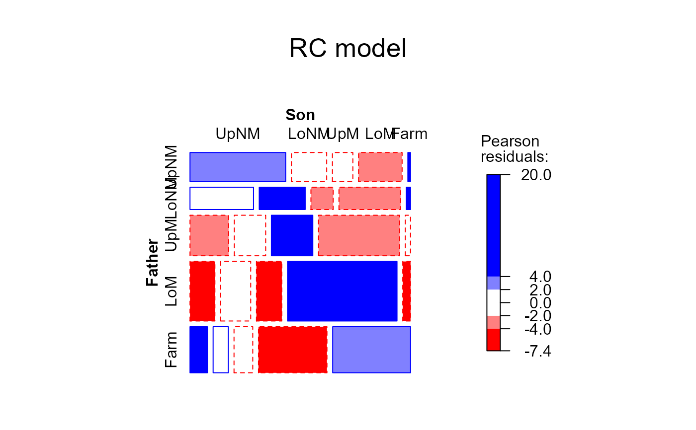 LRstats(hauser.RC)
#> Likelihood summary table:
#> AIC BIC LR Chisq Df Pr(>Chisq)
#> hauser.RC 920.16 939.66 685.45 9 < 2.2e-16 ***
#> ---
#> Signif. codes: 0 ‘***’ 0.001 ‘**’ 0.01 ‘*’ 0.05 ‘.’ 0.1 ‘ ’ 1
# crossings models
hauser.CR <- update(hauser.indep, ~ . + Crossings(Father,Son))
mosaic(hauser.topo, ~Father+Son, main="Crossings model", gp=shading_Friendly)
LRstats(hauser.RC)
#> Likelihood summary table:
#> AIC BIC LR Chisq Df Pr(>Chisq)
#> hauser.RC 920.16 939.66 685.45 9 < 2.2e-16 ***
#> ---
#> Signif. codes: 0 ‘***’ 0.001 ‘**’ 0.01 ‘*’ 0.05 ‘.’ 0.1 ‘ ’ 1
# crossings models
hauser.CR <- update(hauser.indep, ~ . + Crossings(Father,Son))
mosaic(hauser.topo, ~Father+Son, main="Crossings model", gp=shading_Friendly)
 LRstats(hauser.CR)
#> Likelihood summary table:
#> AIC BIC LR Chisq Df Pr(>Chisq)
#> hauser.CR 318.63 334.47 89.914 12 5.131e-14 ***
#> ---
#> Signif. codes: 0 ‘***’ 0.001 ‘**’ 0.01 ‘*’ 0.05 ‘.’ 0.1 ‘ ’ 1
hauser.CRdiag <- update(hauser.indep, ~ . + Crossings(Father,Son) + Diag(Father,Son))
LRstats(hauser.CRdiag)
#> Likelihood summary table:
#> AIC BIC LR Chisq Df Pr(>Chisq)
#> hauser.CRdiag 298.95 318.45 64.237 9 2.03e-10 ***
#> ---
#> Signif. codes: 0 ‘***’ 0.001 ‘**’ 0.01 ‘*’ 0.05 ‘.’ 0.1 ‘ ’ 1
# compare model fit statistics
modlist <- glmlist(hauser.indep, hauser.roweff, hauser.UA, hauser.UAdiag,
hauser.quasi, hauser.qsymm, hauser.topo,
hauser.RC, hauser.CR, hauser.CRdiag)
sumry <- LRstats(modlist)
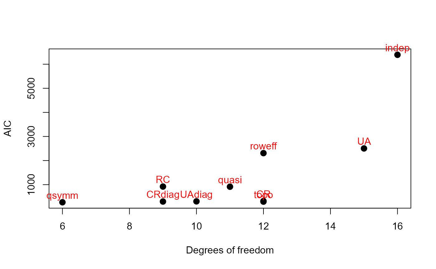
sumry[order(sumry$AIC, decreasing=TRUE),]
#> Likelihood summary table:
#> AIC BIC LR Chisq Df Pr(>Chisq)
#> hauser.indep 6390.8 6401.8 6170.1 16 < 2.2e-16 ***
#> hauser.UA 2503.4 2515.6 2280.7 15 < 2.2e-16 ***
#> hauser.roweff 2308.9 2324.7 2080.2 12 < 2.2e-16 ***
#> hauser.RC 920.2 939.7 685.4 9 < 2.2e-16 ***
#> hauser.quasi 914.1 931.1 683.3 11 < 2.2e-16 ***
#> hauser.CR 318.6 334.5 89.9 12 5.131e-14 ***
#> hauser.UAdiag 305.7 324.0 73.0 10 1.161e-11 ***
#> hauser.CRdiag 298.9 318.5 64.2 9 2.030e-10 ***
#> hauser.topo 295.3 311.1 66.6 12 1.397e-09 ***
#> hauser.qsymm 268.2 291.3 27.4 6 0.0001193 ***
#> ---
#> Signif. codes: 0 ‘***’ 0.001 ‘**’ 0.01 ‘*’ 0.05 ‘.’ 0.1 ‘ ’ 1
# or, more simply
LRstats(modlist, sortby="AIC")
#> Likelihood summary table:
#> AIC BIC LR Chisq Df Pr(>Chisq)
#> hauser.indep 6390.8 6401.8 6170.1 16 < 2.2e-16 ***
#> hauser.UA 2503.4 2515.6 2280.7 15 < 2.2e-16 ***
#> hauser.roweff 2308.9 2324.7 2080.2 12 < 2.2e-16 ***
#> hauser.RC 920.2 939.7 685.4 9 < 2.2e-16 ***
#> hauser.quasi 914.1 931.1 683.3 11 < 2.2e-16 ***
#> hauser.CR 318.6 334.5 89.9 12 5.131e-14 ***
#> hauser.UAdiag 305.7 324.0 73.0 10 1.161e-11 ***
#> hauser.CRdiag 298.9 318.5 64.2 9 2.030e-10 ***
#> hauser.topo 295.3 311.1 66.6 12 1.397e-09 ***
#> hauser.qsymm 268.2 291.3 27.4 6 0.0001193 ***
#> ---
#> Signif. codes: 0 ‘***’ 0.001 ‘**’ 0.01 ‘*’ 0.05 ‘.’ 0.1 ‘ ’ 1
mods <- substring(rownames(sumry),8)
with(sumry,
{plot(Df, AIC, cex=1.3, pch=19, xlab='Degrees of freedom', ylab='AIC')
text(Df, AIC, mods, adj=c(0.5,-.5), col='red', xpd=TRUE)
})
LRstats(hauser.CR)
#> Likelihood summary table:
#> AIC BIC LR Chisq Df Pr(>Chisq)
#> hauser.CR 318.63 334.47 89.914 12 5.131e-14 ***
#> ---
#> Signif. codes: 0 ‘***’ 0.001 ‘**’ 0.01 ‘*’ 0.05 ‘.’ 0.1 ‘ ’ 1
hauser.CRdiag <- update(hauser.indep, ~ . + Crossings(Father,Son) + Diag(Father,Son))
LRstats(hauser.CRdiag)
#> Likelihood summary table:
#> AIC BIC LR Chisq Df Pr(>Chisq)
#> hauser.CRdiag 298.95 318.45 64.237 9 2.03e-10 ***
#> ---
#> Signif. codes: 0 ‘***’ 0.001 ‘**’ 0.01 ‘*’ 0.05 ‘.’ 0.1 ‘ ’ 1
# compare model fit statistics
modlist <- glmlist(hauser.indep, hauser.roweff, hauser.UA, hauser.UAdiag,
hauser.quasi, hauser.qsymm, hauser.topo,
hauser.RC, hauser.CR, hauser.CRdiag)
sumry <- LRstats(modlist)
sumry[order(sumry$AIC, decreasing=TRUE),]
#> Likelihood summary table:
#> AIC BIC LR Chisq Df Pr(>Chisq)
#> hauser.indep 6390.8 6401.8 6170.1 16 < 2.2e-16 ***
#> hauser.UA 2503.4 2515.6 2280.7 15 < 2.2e-16 ***
#> hauser.roweff 2308.9 2324.7 2080.2 12 < 2.2e-16 ***
#> hauser.RC 920.2 939.7 685.4 9 < 2.2e-16 ***
#> hauser.quasi 914.1 931.1 683.3 11 < 2.2e-16 ***
#> hauser.CR 318.6 334.5 89.9 12 5.131e-14 ***
#> hauser.UAdiag 305.7 324.0 73.0 10 1.161e-11 ***
#> hauser.CRdiag 298.9 318.5 64.2 9 2.030e-10 ***
#> hauser.topo 295.3 311.1 66.6 12 1.397e-09 ***
#> hauser.qsymm 268.2 291.3 27.4 6 0.0001193 ***
#> ---
#> Signif. codes: 0 ‘***’ 0.001 ‘**’ 0.01 ‘*’ 0.05 ‘.’ 0.1 ‘ ’ 1
# or, more simply
LRstats(modlist, sortby="AIC")
#> Likelihood summary table:
#> AIC BIC LR Chisq Df Pr(>Chisq)
#> hauser.indep 6390.8 6401.8 6170.1 16 < 2.2e-16 ***
#> hauser.UA 2503.4 2515.6 2280.7 15 < 2.2e-16 ***
#> hauser.roweff 2308.9 2324.7 2080.2 12 < 2.2e-16 ***
#> hauser.RC 920.2 939.7 685.4 9 < 2.2e-16 ***
#> hauser.quasi 914.1 931.1 683.3 11 < 2.2e-16 ***
#> hauser.CR 318.6 334.5 89.9 12 5.131e-14 ***
#> hauser.UAdiag 305.7 324.0 73.0 10 1.161e-11 ***
#> hauser.CRdiag 298.9 318.5 64.2 9 2.030e-10 ***
#> hauser.topo 295.3 311.1 66.6 12 1.397e-09 ***
#> hauser.qsymm 268.2 291.3 27.4 6 0.0001193 ***
#> ---
#> Signif. codes: 0 ‘***’ 0.001 ‘**’ 0.01 ‘*’ 0.05 ‘.’ 0.1 ‘ ’ 1
mods <- substring(rownames(sumry),8)
with(sumry,
{plot(Df, AIC, cex=1.3, pch=19, xlab='Degrees of freedom', ylab='AIC')
text(Df, AIC, mods, adj=c(0.5,-.5), col='red', xpd=TRUE)
})