Association Graph for a Loglinear Model

Construct an undirected graph representing the associations in a loglinear model. Nodes represent variables and edges represent pairwise associations fitted in the model. If two variables are not connected by an edge, they are conditionally independent given the other variables.

Usage

assoc_graph(x, ...)

# S3 method for class 'list'
assoc_graph(x, result = c("igraph", "matrix", "edge_list"), ...)

# S3 method for class 'loglm'
assoc_graph(x, result = c("igraph", "matrix", "edge_list"), ...)

# S3 method for class 'glm'
assoc_graph(
  x,
  result = c("igraph", "matrix", "edge_list"),
  measure = c("none", "chisq", "cramer"),
  ...
)

# S3 method for class 'assoc_graph'
print(x, ...)

Arguments

x

An object specifying the model. Can be:

A list of character vectors (a margin/generating class list, as produced by joint, conditional, etc.)
A fitted loglm object
A fitted glm object (poisson family loglinear model)

...

Additional arguments (currently unused).

result

Type of result to return: "igraph" (default) returns an igraph object; "matrix" returns the adjacency matrix; "edge_list" returns a two-column character matrix of edges.

measure

Type of association measure for edge weights (only for glm method): "none" (default) produces an unweighted graph; "chisq" computes partial chi-squared statistics (deviance change when each edge is removed from the model); "cramer" computes Cramer's V from the marginal two-way table for each edge.

Value

Depending on result:

"igraph": An igraph undirected graph object of class c("assoc_graph", "igraph"), with vertex names corresponding to the variable names. When measure != "none", edge weights are stored as E(g)$weight and the measure name as g$measure.
"matrix": A symmetric adjacency matrix with variable names as row and column names. Contains 0/1 when unweighted, or association strength values when measure is specified.
"edge_list": When unweighted, a two-column character matrix (from, to). When measure is specified, a data frame with columns from, to, and weight.

Details

Each high-order term (margin) in a hierarchical loglinear model defines a clique in the association graph. For example, the term c("A", "B", "C") generates edges A–B, A–C, and B–C. Single-variable terms (as in mutual independence) yield isolated nodes with no edges.

For loglm objects, the margins are extracted from the $margin component. For glm objects, the interaction terms are extracted from the model formula.

References

Khamis, H. J. (2011). The Association Graph and the Multigraph for Loglinear Models. SAGE Publications. doi:10.4135/9781452226521

Darroch, J. N., Lauritzen, S. L., & Speed, T. P. (1980). Markov Fields and Log-Linear Interaction Models for Contingency Tables. The Annals of Statistics, 8(3), 522–539. doi:10.1214/aos/1176345006

Whittaker, J. (1990). Graphical Models in Applied Multivariate Statistics. John Wiley & Sons, Chichester.

Examples

# Structural graphs from margin lists (3-way: A, B, C)
mutual(3, factors = c("A", "B", "C"))      |> assoc_graph()
#> Association graph: 3 variables, 0 edges
#> Variables: A, B, C 
#> Edges: (none -- mutual independence)
#> Model: [A] [B] [C] 
joint(3, factors = c("A", "B", "C"))       |> assoc_graph()
#> Association graph: 3 variables, 1 edges
#> Variables: A, B, C 
#> Edges: A -- B 
#> Model: [C] [A,B] 
conditional(3, factors = c("A", "B", "C")) |> assoc_graph()
#> Association graph: 3 variables, 2 edges
#> Variables: A, C, B 
#> Edges: A -- C, C -- B 
#> Model: [A,C] [C,B] 
saturated(3, factors = c("A", "B", "C"))   |> assoc_graph()
#> Association graph: 3 variables, 3 edges
#> Variables: A, B, C 
#> Edges: A -- B, A -- C, B -- C 
#> Model: [A,B,C] 

# Adjacency matrix form
conditional(3, factors = c("A", "B", "C")) |> assoc_graph(result = "matrix")
#>   A C B
#> A 0 1 0
#> C 1 0 1
#> B 0 1 0

# From a fitted loglm model (Berkeley admissions)
if (FALSE) { # \dontrun{
mod <- MASS::loglm(~ (Admit + Gender) * Dept, data = UCBAdmissions)
assoc_graph(mod)
plot(assoc_graph(mod), main = "Berkeley: [AD] [GD]")
} # }

# From glm models (Dayton Survey: cigarette, alcohol, marijuana, sex, race)
data(DaytonSurvey)

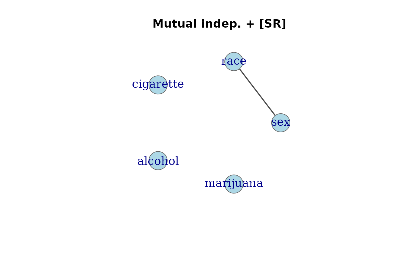
# Mutual independence + sex*race: one edge only
mod.SR <- glm(Freq ~ . + sex*race, data = DaytonSurvey, family = poisson)
assoc_graph(mod.SR)
#> Association graph: 5 variables, 1 edges
#> Variables: sex, race, cigarette, alcohol, marijuana 
#> Edges: sex -- race 
#> Model: [cigarette] [alcohol] [marijuana] [sex,race] 
plot(assoc_graph(mod.SR), main = "Mutual indep. + [SR]")


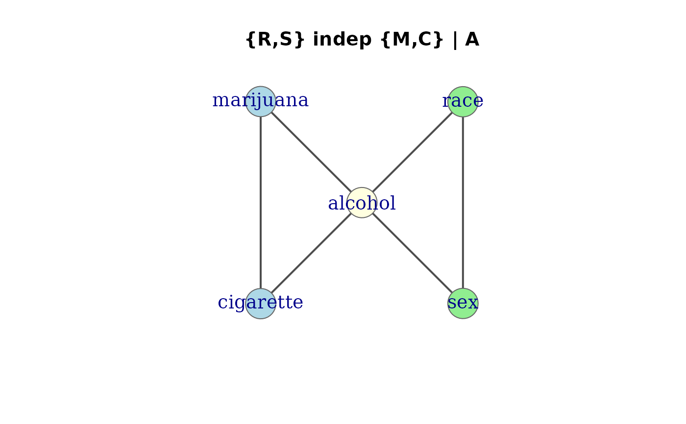
# [AM][AC][MC][AR][AS][RS]: {race, sex} indep {marijuana, cigs} | alcohol
mod.cond <- glm(Freq ~ (cigarette + alcohol + marijuana)^2 +
                        (alcohol + sex + race)^2,
                data = DaytonSurvey, family = poisson)

# define groups for the model
gps <- list(c("cigarette", "marijuana"),
            "alcohol",
            c("sex", "race"))

assoc_graph(mod.cond)
#> Association graph: 5 variables, 6 edges
#> Variables: cigarette, alcohol, marijuana, sex, race 
#> Edges: cigarette -- alcohol, cigarette -- marijuana, alcohol -- marijuana, alcohol -- sex, alcohol -- race, sex -- race 
#> Model: [cigarette,alcohol,marijuana] [alcohol,sex,race] 
plot(assoc_graph(mod.cond),
     groups = gps,
     layout = igraph::layout_nicely,
     main = "{R,S} indep {M,C} | A")


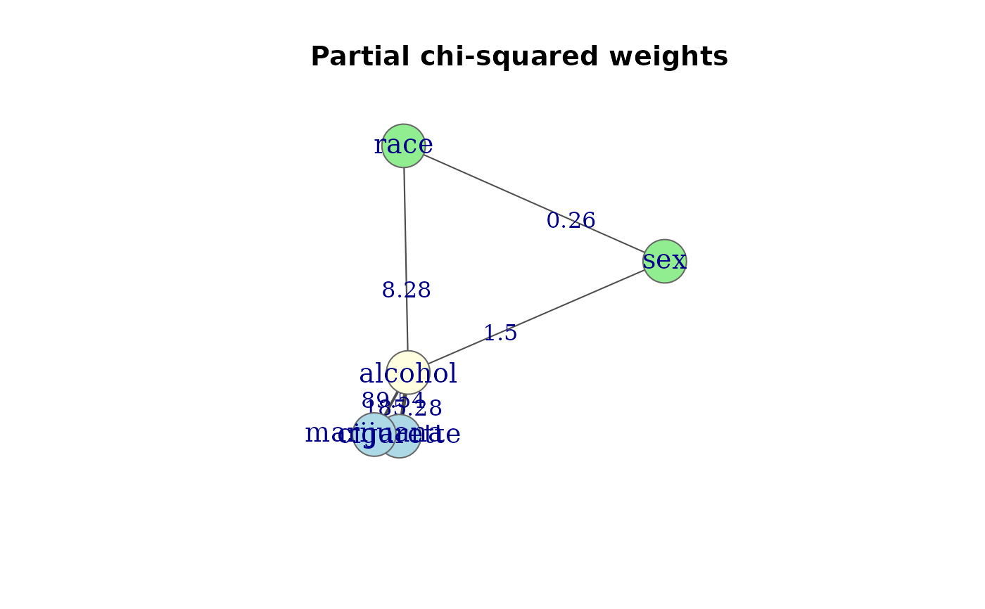
# Weighted graph: partial chi-squared
g <- assoc_graph(mod.cond, measure = "chisq")
g
#> Association graph: 5 variables, 6 edges
#> Variables: cigarette, alcohol, marijuana, sex, race 
#> Edges: cigarette -- alcohol (185.28), cigarette -- marijuana (494.9), alcohol -- marijuana (89.54), alcohol -- sex (1.5), alcohol -- race (8.28), sex -- race (0.26) 
#> Measure: chisq 
#> Model: [cigarette,alcohol,marijuana] [alcohol,sex,race] 
plot(g, edge.label = TRUE,
     groups = gps,
     layout = igraph::layout_nicely,
     main = "Partial chi-squared weights")


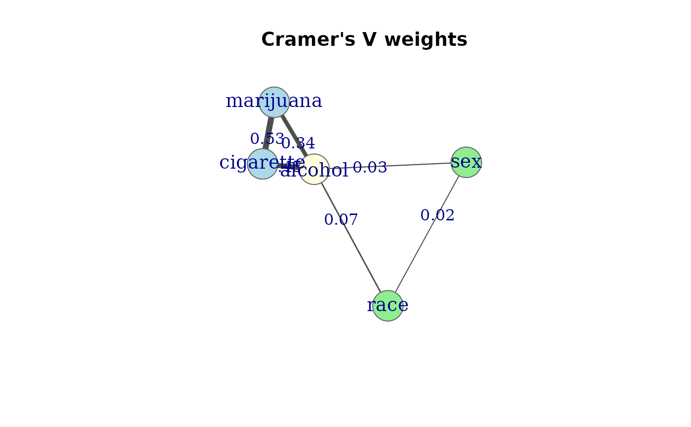
# Cramer's V (marginal)
g2 <- assoc_graph(mod.cond, measure = "cramer")
g2
#> Association graph: 5 variables, 6 edges
#> Variables: cigarette, alcohol, marijuana, sex, race 
#> Edges: cigarette -- alcohol (0.45), cigarette -- marijuana (0.53), alcohol -- marijuana (0.34), alcohol -- sex (0.03), alcohol -- race (0.07), sex -- race (0.02) 
#> Measure: cramer 
#> Model: [cigarette,alcohol,marijuana] [alcohol,sex,race] 
plot(g2, edge.label = TRUE,
     groups = gps,
     layout = igraph::layout_nicely,
     main = "Cramer's V weights")