The dataset NLSY comes from a small part of the National Longitudinal Survey of
Youth, which is a series of annual surveys conducted by the
U.S. Department of Labor to examine the transition of young people into the labor force.
This particular subset gives measures of 243 children on mathematics and reading achievement and also
measures of behavioral problems (antisocial, hyperactivity). Also available are the yearly income
and education of the child's father.
Format
A data frame with 243 observations on the following 6 variables.
mathMath achievement test score
readReading achievement test score
antisocscore on a measure of child's antisocial behavior,
0:6hyperactscore on a measure of child's hyperactive behavior,
0:5incomeyearly income of child's father
educyears of education of child's father
Source
This dataset was derived from a larger one used by Patrick Curran at the 1997 meeting of the Society for Research on Child Development (SRCD). A description now only exists on the WayBack Machine, http://web.archive.org/web/20050404145001/http://www.unc.edu/~curran/example.html.
More details are available at http://web.archive.org/web/20060830061414/http://www.unc.edu/~curran/srcd-docs/srcdmeth.pdf.
Details
For the examples using this dataset, math and read scores are taken at the outcome
variables. Among the remaining predictors, income and educ
might be considered as background variables necessary to control for.
Interest might then be focused on whether the behavioral variables
antisoc and hyperact contribute beyond that.
The distribution of father's income is very highly skewed in the positive direction.
Linear model analysis should probably use log(income), but this is omitted for simplicity.
The dataset also contains a few unusual observations for you to discover.
Examples
library(car)
data(NLSY)
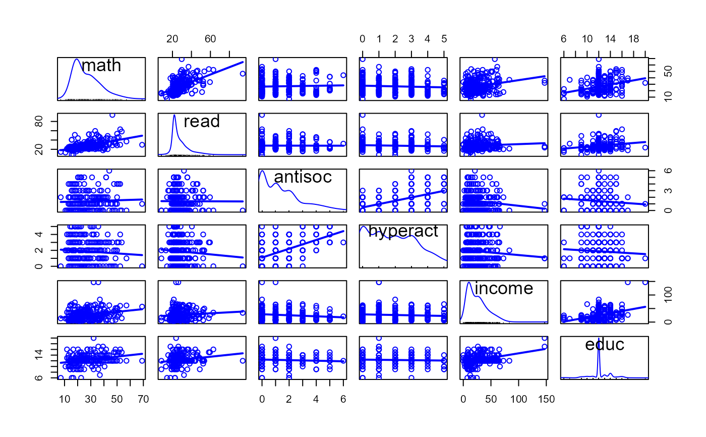
#examine the data
scatterplotMatrix(NLSY, smooth=FALSE)
 # test control variables by themselves
# -------------------------------------
NLSY.mod1 <- lm(cbind(read, math) ~ income + educ, data=NLSY)
Anova(NLSY.mod1)
#>
#> Type II MANOVA Tests: Pillai test statistic
#> Df test stat approx F num Df den Df Pr(>F)
#> income 1 0.034469 4.2661 2 239 0.015121 *
#> educ 1 0.051521 6.4912 2 239 0.001798 **
#> ---
#> Signif. codes: 0 '***' 0.001 '**' 0.01 '*' 0.05 '.' 0.1 ' ' 1
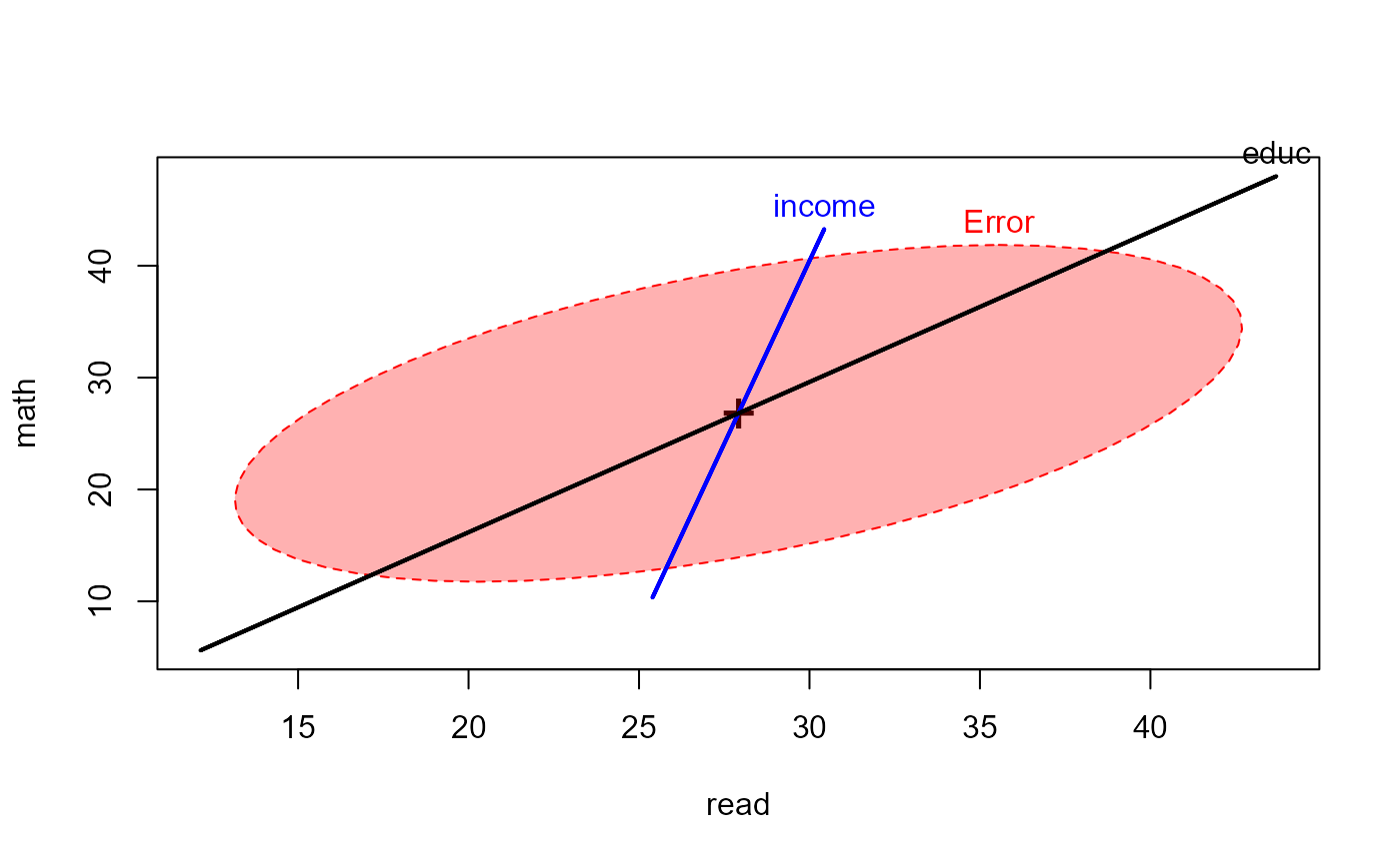
heplot(NLSY.mod1, fill=TRUE)
# test control variables by themselves
# -------------------------------------
NLSY.mod1 <- lm(cbind(read, math) ~ income + educ, data=NLSY)
Anova(NLSY.mod1)
#>
#> Type II MANOVA Tests: Pillai test statistic
#> Df test stat approx F num Df den Df Pr(>F)
#> income 1 0.034469 4.2661 2 239 0.015121 *
#> educ 1 0.051521 6.4912 2 239 0.001798 **
#> ---
#> Signif. codes: 0 '***' 0.001 '**' 0.01 '*' 0.05 '.' 0.1 ' ' 1
heplot(NLSY.mod1, fill=TRUE)
 # test of overall regression
coefs <- rownames(coef(NLSY.mod1))[-1]
linearHypothesis(NLSY.mod1, coefs)
#>
#> Sum of squares and products for the hypothesis:
#> read math
#> read 859.6586 1474.716
#> math 1474.7164 2929.558
#>
#> Sum of squares and products for error:
#> read math
#> read 22882.46 12051.69
#> math 12051.69 23763.79
#>
#> Multivariate Tests:
#> Df test stat approx F num Df den Df Pr(>F)
#> Pillai 2 0.1166962 7.435629 4 480 8.1261e-06 ***
#> Wilks 2 0.8840660 7.594147 4 478 6.1527e-06 ***
#> Hotelling-Lawley 2 0.1302750 7.751361 4 476 4.6699e-06 ***
#> Roy 2 0.1232808 14.793699 2 240 8.7377e-07 ***
#> ---
#> Signif. codes: 0 '***' 0.001 '**' 0.01 '*' 0.05 '.' 0.1 ' ' 1
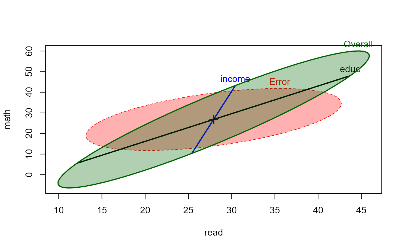
heplot(NLSY.mod1, fill=TRUE, hypotheses=list("Overall"=coefs))
# test of overall regression
coefs <- rownames(coef(NLSY.mod1))[-1]
linearHypothesis(NLSY.mod1, coefs)
#>
#> Sum of squares and products for the hypothesis:
#> read math
#> read 859.6586 1474.716
#> math 1474.7164 2929.558
#>
#> Sum of squares and products for error:
#> read math
#> read 22882.46 12051.69
#> math 12051.69 23763.79
#>
#> Multivariate Tests:
#> Df test stat approx F num Df den Df Pr(>F)
#> Pillai 2 0.1166962 7.435629 4 480 8.1261e-06 ***
#> Wilks 2 0.8840660 7.594147 4 478 6.1527e-06 ***
#> Hotelling-Lawley 2 0.1302750 7.751361 4 476 4.6699e-06 ***
#> Roy 2 0.1232808 14.793699 2 240 8.7377e-07 ***
#> ---
#> Signif. codes: 0 '***' 0.001 '**' 0.01 '*' 0.05 '.' 0.1 ' ' 1
heplot(NLSY.mod1, fill=TRUE, hypotheses=list("Overall"=coefs))
 # coefficient plot
coefplot(NLSY.mod1, fill = TRUE,
col = c("darkgreen", "brown"),
lwd = 2,
ylim = c(-0.5, 3),
main = "Bivariate coefficient plot for reading and math\nwith 95% confidence ellipses")
# coefficient plot
coefplot(NLSY.mod1, fill = TRUE,
col = c("darkgreen", "brown"),
lwd = 2,
ylim = c(-0.5, 3),
main = "Bivariate coefficient plot for reading and math\nwith 95% confidence ellipses")
 # additional contribution of antisoc + hyperact over income + educ
# ----------------------------------------------------------------
NLSY.mod2 <- lm(cbind(read,math) ~ antisoc + hyperact + income + educ, data=NLSY)
Anova(NLSY.mod2)
#>
#> Type II MANOVA Tests: Pillai test statistic
#> Df test stat approx F num Df den Df Pr(>F)
#> antisoc 1 0.019343 2.3374 2 237 0.098803 .
#> hyperact 1 0.014442 1.7364 2 237 0.178380
#> income 1 0.038280 4.7167 2 237 0.009801 **
#> educ 1 0.053152 6.6521 2 237 0.001546 **
#> ---
#> Signif. codes: 0 '***' 0.001 '**' 0.01 '*' 0.05 '.' 0.1 ' ' 1
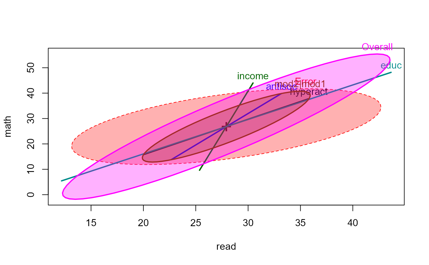
coefs <- rownames(coef(NLSY.mod2))[-1]
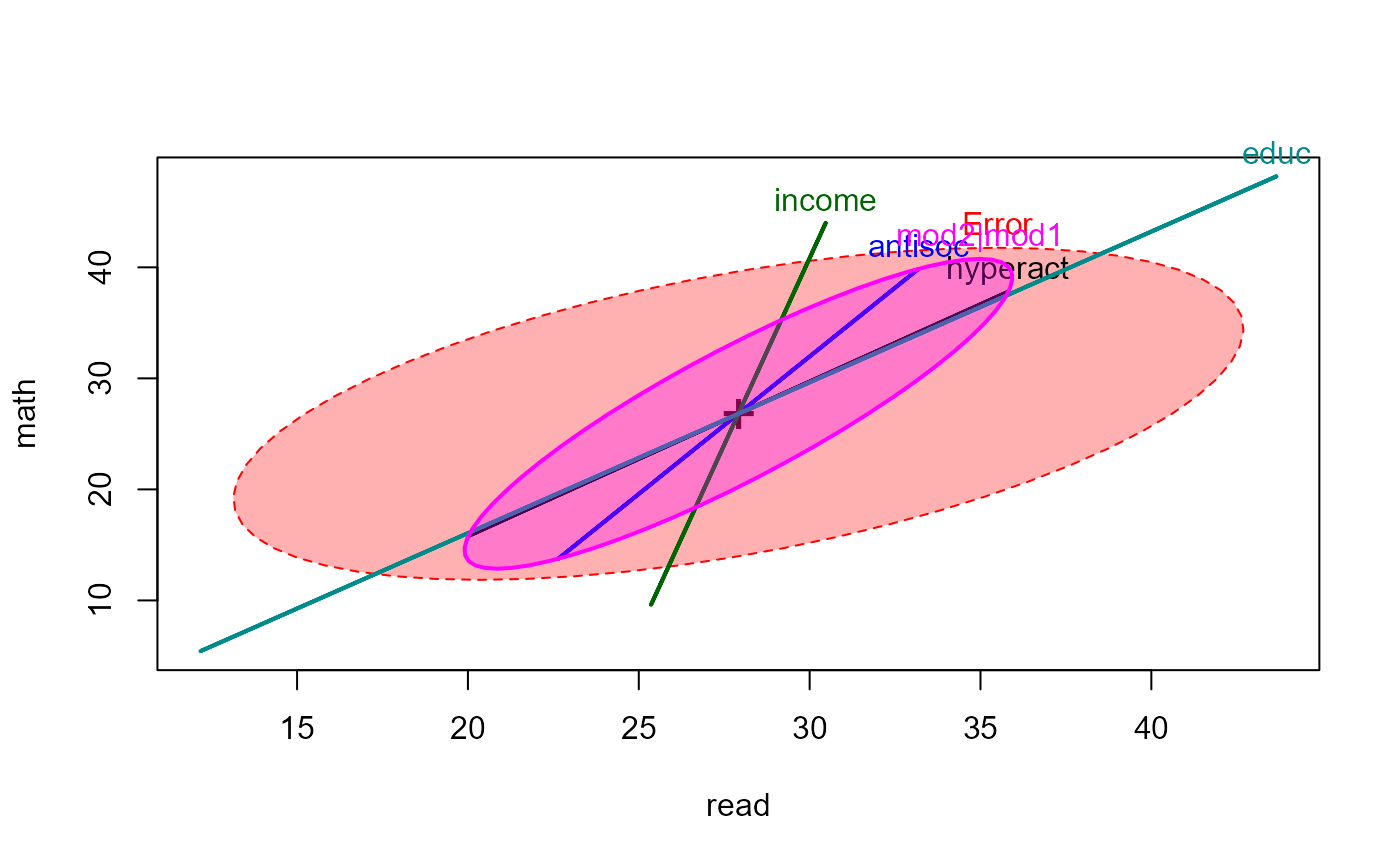
heplot(NLSY.mod2, fill=TRUE, hypotheses=list("Overall"=coefs, "mod2|mod1"=coefs[1:2]))
# additional contribution of antisoc + hyperact over income + educ
# ----------------------------------------------------------------
NLSY.mod2 <- lm(cbind(read,math) ~ antisoc + hyperact + income + educ, data=NLSY)
Anova(NLSY.mod2)
#>
#> Type II MANOVA Tests: Pillai test statistic
#> Df test stat approx F num Df den Df Pr(>F)
#> antisoc 1 0.019343 2.3374 2 237 0.098803 .
#> hyperact 1 0.014442 1.7364 2 237 0.178380
#> income 1 0.038280 4.7167 2 237 0.009801 **
#> educ 1 0.053152 6.6521 2 237 0.001546 **
#> ---
#> Signif. codes: 0 '***' 0.001 '**' 0.01 '*' 0.05 '.' 0.1 ' ' 1
coefs <- rownames(coef(NLSY.mod2))[-1]
heplot(NLSY.mod2, fill=TRUE, hypotheses=list("Overall"=coefs, "mod2|mod1"=coefs[1:2]))
 linearHypothesis(NLSY.mod2, coefs[1:2])
#>
#> Sum of squares and products for the hypothesis:
#> read math
#> read 170.3478 261.2230
#> math 261.2230 516.0188
#>
#> Sum of squares and products for error:
#> read math
#> read 22712.12 11790.46
#> math 11790.46 23247.77
#>
#> Multivariate Tests:
#> Df test stat approx F num Df den Df Pr(>F)
#> Pillai 2 0.0239869 1.444548 4 476 0.218172
#> Wilks 2 0.9760624 1.444284 4 474 0.218264
#> Hotelling-Lawley 2 0.0244741 1.443972 4 472 0.218372
#> Roy 2 0.0221965 2.641385 2 238 0.073351 .
#> ---
#> Signif. codes: 0 '***' 0.001 '**' 0.01 '*' 0.05 '.' 0.1 ' ' 1
heplot(NLSY.mod2, fill=TRUE, hypotheses=list("mod2|mod1"=coefs[1:2]))
linearHypothesis(NLSY.mod2, coefs[1:2])
#>
#> Sum of squares and products for the hypothesis:
#> read math
#> read 170.3478 261.2230
#> math 261.2230 516.0188
#>
#> Sum of squares and products for error:
#> read math
#> read 22712.12 11790.46
#> math 11790.46 23247.77
#>
#> Multivariate Tests:
#> Df test stat approx F num Df den Df Pr(>F)
#> Pillai 2 0.0239869 1.444548 4 476 0.218172
#> Wilks 2 0.9760624 1.444284 4 474 0.218264
#> Hotelling-Lawley 2 0.0244741 1.443972 4 472 0.218372
#> Roy 2 0.0221965 2.641385 2 238 0.073351 .
#> ---
#> Signif. codes: 0 '***' 0.001 '**' 0.01 '*' 0.05 '.' 0.1 ' ' 1
heplot(NLSY.mod2, fill=TRUE, hypotheses=list("mod2|mod1"=coefs[1:2]))
 # check for outliers
idx <- cqplot(NLSY.mod2, id.n = 5)
# check for outliers
idx <- cqplot(NLSY.mod2, id.n = 5)
 idx
#> DSQ quantile p
#> 142 49.21118 12.372417 0.002057613
#> 12 20.58795 10.175193 0.006172840
#> 152 11.61444 9.153541 0.010288066
#> 124 11.27507 8.480597 0.014403292
#> 102 11.13109 7.977968 0.018518519
idx
#> DSQ quantile p
#> 142 49.21118 12.372417 0.002057613
#> 12 20.58795 10.175193 0.006172840
#> 152 11.61444 9.153541 0.010288066
#> 124 11.27507 8.480597 0.014403292
#> 102 11.13109 7.977968 0.018518519