Coefficient plots for Multivariate Linear Models

Displays bivariate confidence ellipses for all parameters in an multivariate linear model, for a given pair of variables. In contrast to univariate coefficient plots for an ordinary linear model (e.g., parameters::model_parameters(), plotted via its plot() method), which show confidence intervals for parameters one at a time, these plots show how each predictor moves a pair of responses jointly, in a way that can readily be compared.

Usage

coefplot(object, ...)

# S3 method for class 'mlm'
coefplot(
  object,
  variables = 1:2,
  parm = NULL,
  df = NULL,
  level = 0.95,
  intercept = FALSE,
  std = FALSE,
  Scheffe = FALSE,
  bars = TRUE,
  fill = FALSE,
  fill.alpha = 0.2,
  labels = !add,
  label.pos = NULL,
  xlab,
  ylab,
  xlim = NULL,
  ylim = NULL,
  axes = TRUE,
  main = "",
  add = FALSE,
  lwd = 1,
  lty = 1,
  pch = 19,
  col = palette(),
  cex = 2,
  cex.label = 1.5,
  cex.lab = par("cex.lab"),
  lty.zero = 3,
  col.zero = 1,
  pch.zero = "+",
  verbose = FALSE,
  ...
)

Arguments

object: A multivariate linear model, such as fit by lm(cbind(y1, y2, ...) ~ terms, ...)
...: Other parameters passed to graphics::plot()
variables: Response variables to plot, given as their indices or names
parm: Parameters to plot, given as their indices or names
df: Degrees of freedom for hypothesis tests
level: Confidence level for the confidence ellipses
intercept: logical. Include the intercept?
std: logical. If TRUE, plot standardized coefficients instead – see stdmodel() for the standardization convention (response(s) and numeric predictors are standardized; factor predictors are left on their raw 0/1 scale). Not generally useful together with intercept = TRUE, since the intercept becomes ~0 once standardized.
Scheffe: If TRUE, confidence intervals for all parameters have Scheffe coverage, otherwise, individual coverage.
bars: Draw univariate confidence intervals for each of the variables?
fill: a logical value or vector. TRUE means the confidence ellipses will be filled.
fill.alpha: Opacity of the confidence ellipses
labels: Labels for the confidence ellipses
label.pos: Positions of the labels for each ellipse. See label.ellipse()
xlab, ylab: x, y axis labels
xlim, ylim: Axis limits
axes: Draw axes?
main: Plot title
add: logical. Add to an existing plot?
lwd: Line widths
lty: Line types
pch: Point symbols for the parameter estimates
col: Colors for the confidence ellipses, points, lines
cex: Character size for points showing parameter estimates
cex.label: Character size for ellipse labels
cex.lab: Character size for axis labels. Defaults to par("cex.lab").
lty.zero, col.zero, pch.zero: Line type, color and point symbol for horizontal and vertical lines at 0, 0. These default to lty.zero = 3, col.zero = 1 (black) and pch.zero = '+'.
verbose: logical. Print parameter estimates and variance-covariance for each parameter?

Value

Returns invisibly a list of the coordinates of the ellipses drawn

Details

This function is also a generalization of car::confidenceEllipse() to a multivariate setting. Note that confidenceEllipse() also has an mlm method (via car::confidenceEllipse()), but it answers a different question: it fixes a pair of coefficients (for one or more responses) as the plot axes, and shows their joint confidence region. coefplot() instead fixes a pair of responses as the axes and overlays one ellipse per predictor – use it when the question is "how does each predictor move these two responses together?", and confidenceEllipse() when the question is about the relationship between two specific coefficients.

Author

Michael Friendly

Examples


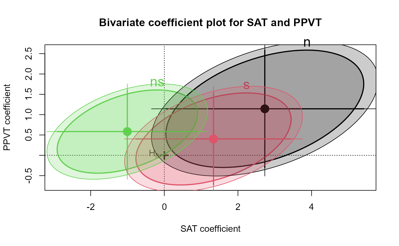
rohwer.mlm <- lm(cbind(SAT,PPVT,Raven)~n+s+ns, data=Rohwer)

coefplot(rohwer.mlm, lwd=2, 
         main="Bivariate coefficient plot for SAT and PPVT", fill=TRUE)
coefplot(rohwer.mlm, add=TRUE, Scheffe=TRUE, fill=TRUE)


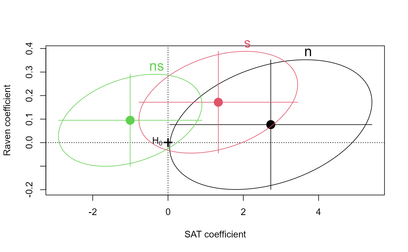
coefplot(rohwer.mlm, var=c(1,3))


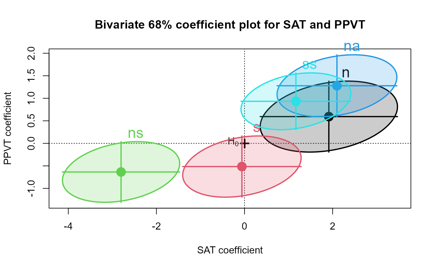
mod1 <- lm(cbind(SAT,PPVT,Raven)~n+s+ns+na+ss, data=Rohwer)
coefplot(mod1, lwd=2, fill=TRUE, parm=(1:5),
  main="Bivariate 68% coefficient plot for SAT and PPVT", level=0.68)


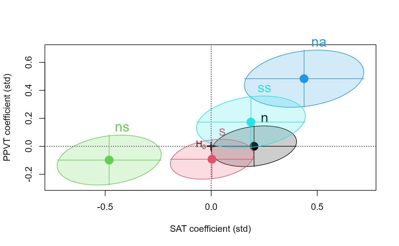
# standardized coefficients, with a factor predictor (SES) in the model
# but excluded from the plotted parm range
mod2 <- lm(cbind(SAT,PPVT,Raven) ~ SES+n+s+ns+na+ss, data=Rohwer)
coefplot(mod2, parm=2:6, std=TRUE, fill=TRUE, level=0.68)