Dogfood Preferences — dogfood • heplots

A tiny hypothetical dataset to illustrate one-way MANOVA.

A dogfood manufacturer wanted to study preference for different dogfood formulas, two of their own ("Old", "New") and two from other manufacturers ("Major", "Alps"). In a between-dog design, 4 dogs were presented with a bowl of one formula and the time to start eating and amount eaten were recorded.

Usage

data("dogfood")

Format

A data frame with 16 observations on the following 3 variables.

formula: factor, a factor with levels Old, New, Major, Alps
start: numeric, time to start eating
amount: numeric, amount eaten

Source

Used in my Psych 6140 lecture notes, http://friendly.apps01.yorku.ca/psy6140/

Details

In addition to testing the overall effects of formula, three useful (and orthogonal) contrasts can specified for this 3-df factor:

Ours vs. Theirs, with weights c(1, 1, -1, -1)
Major vs. Alps, with weights c(0, 0, 1, -1)
Old vs. New, with weights c(1, -1, 0, 0)

Because these are orthogonal contrasts, they fully decompose the main effect of formula, in that their sum of squares add to the overall sum of squares.

Examples

data(dogfood)
library(car)
library(candisc)
#> 
#> Attaching package: 'candisc'
#> The following object is masked from 'package:stats':
#> 
#>     cancor

# make some boxplots
op <- par(mfrow = c(1,2))
boxplot(start ~ formula, data = dogfood)
points(start ~ formula, data = dogfood, pch=16, cex = 1.2)

boxplot(amount ~ formula, data = dogfood)
points(amount ~ formula, data = dogfood, pch=16, cex = 1.2)

par(op)

# setup contrasts to test interesting comparisons
C <- matrix(
       c( 1,  1, -1, -1,         #Ours vs. Theirs
          0,  0,  1, -1,           #Major vs. Alps
          1, -1,  0,  0),             #New vs. Old
       nrow=4, ncol=3)
# assign these to the formula factor
contrasts(dogfood$formula) <- C
# re-fit the model
dogfood.mod <- lm(cbind(start, amount) ~ formula, data=dogfood)

dogfood.mod <- lm(cbind(start, amount) ~ formula, data=dogfood)
Anova(dogfood.mod)
#> 
#> Type II MANOVA Tests: Pillai test statistic
#>         Df test stat approx F num Df den Df  Pr(>F)  
#> formula  3   0.70178   2.1623      6     24 0.08289 .
#> ---
#> Signif. codes:  0 '***' 0.001 '**' 0.01 '*' 0.05 '.' 0.1 ' ' 1

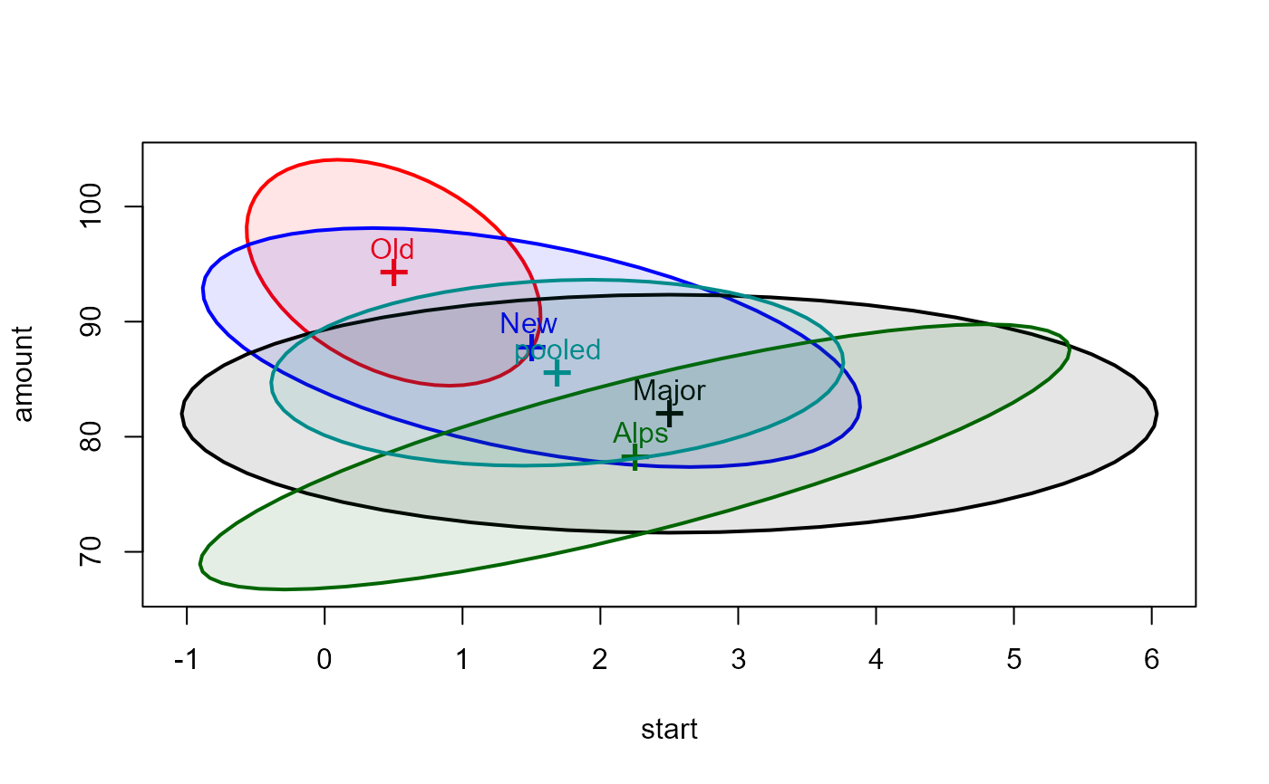
# data ellipses
covEllipses(cbind(start, amount) ~ formula, data=dogfood,
  fill = TRUE, fill.alpha = 0.1)


# test these contrasts with multivariate tests 
linearHypothesis(dogfood.mod, "formula1", title="Ours vs. Theirs")
#> 
#> Sum of squares and products for the hypothesis:
#>           start   amount
#> start    7.5625 -59.8125
#> amount -59.8125 473.0625
#> 
#> Sum of squares and products for error:
#>        start amount
#> start  25.75  11.75
#> amount 11.75 390.25
#> 
#> Multivariate Tests: Ours vs. Theirs
#>                  Df test stat approx F num Df den Df    Pr(>F)   
#> Pillai            1 0.6252849 9.177818      2     11 0.0045223 **
#> Wilks             1 0.3747151 9.177818      2     11 0.0045223 **
#> Hotelling-Lawley  1 1.6686941 9.177818      2     11 0.0045223 **
#> Roy               1 1.6686941 9.177818      2     11 0.0045223 **
#> ---
#> Signif. codes:  0 '***' 0.001 '**' 0.01 '*' 0.05 '.' 0.1 ' ' 1
linearHypothesis(dogfood.mod, "formula2", title="Old vs. New")
#> 
#> Sum of squares and products for the hypothesis:
#>        start amount
#> start  0.125  1.875
#> amount 1.875 28.125
#> 
#> Sum of squares and products for error:
#>        start amount
#> start  25.75  11.75
#> amount 11.75 390.25
#> 
#> Multivariate Tests: Old vs. New
#>                  Df test stat  approx F num Df den Df  Pr(>F)
#> Pillai            1 0.0685104 0.4045209      2     11 0.67683
#> Wilks             1 0.9314896 0.4045209      2     11 0.67683
#> Hotelling-Lawley  1 0.0735493 0.4045209      2     11 0.67683
#> Roy               1 0.0735493 0.4045209      2     11 0.67683
linearHypothesis(dogfood.mod, "formula3", title="Alps vs. Major")
#> 
#> Sum of squares and products for the hypothesis:
#>        start amount
#> start      2  -13.0
#> amount   -13   84.5
#> 
#> Sum of squares and products for error:
#>        start amount
#> start  25.75  11.75
#> amount 11.75 390.25
#> 
#> Multivariate Tests: Alps vs. Major
#>                  Df test stat approx F num Df den Df  Pr(>F)
#> Pillai            1 0.2476229 1.810164      2     11 0.20912
#> Wilks             1 0.7523771 1.810164      2     11 0.20912
#> Hotelling-Lawley  1 0.3291208 1.810164      2     11 0.20912
#> Roy               1 0.3291208 1.810164      2     11 0.20912

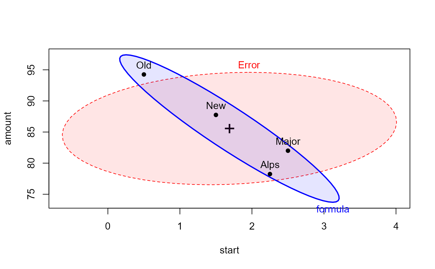
heplot(dogfood.mod, fill = TRUE, fill.alpha = 0.1)


# display contrasts in the heplot 
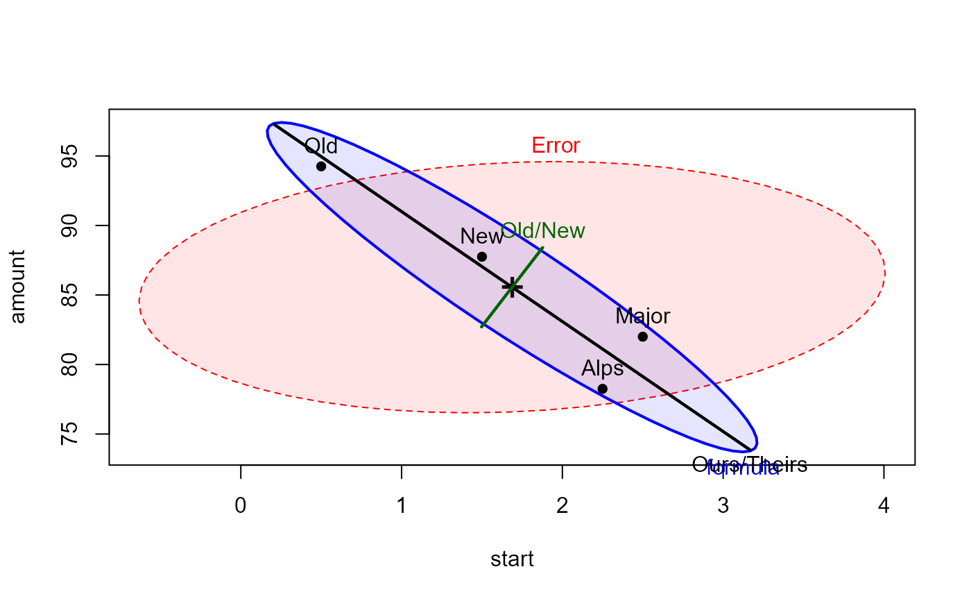
hyp <- list("Ours/Theirs" = "formula1",
            "Old/New" = "formula2")
heplot(dogfood.mod, hypotheses = hyp,
       fill = TRUE, fill.alpha = 0.1)


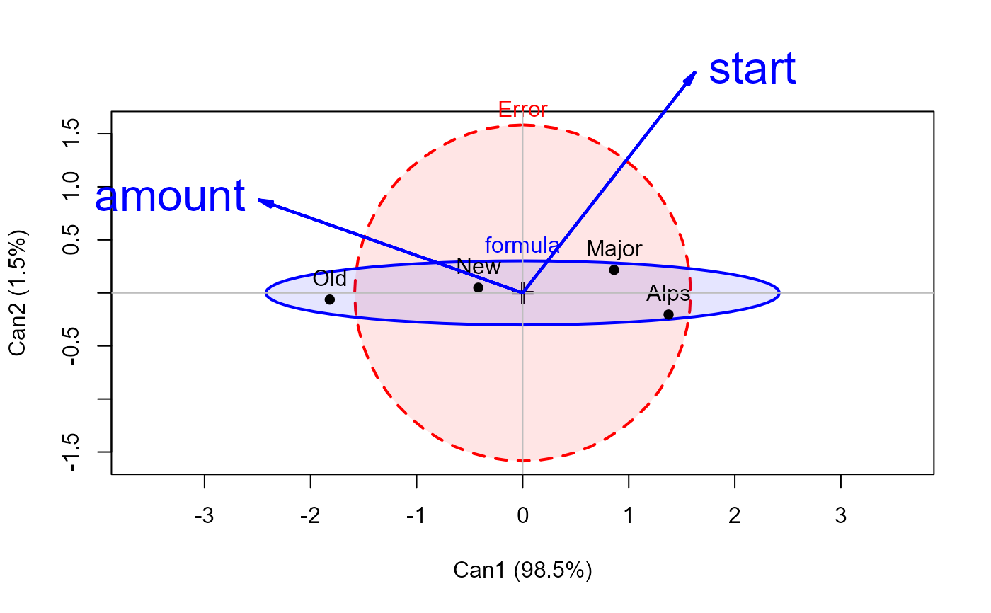dogfood.can <- candisc(dogfood.mod, data=dogfood)
heplot(dogfood.can, 
       fill = TRUE, fill.alpha = 0.1, 
       lwd = 2, var.lwd = 2, var.cex = 2)

#> Vector scale factor set to  2.635145